miniTE Technical Report: Stable and Efficient Reinforcement Learning with Native NVFP4
ABSTRACT
Native NVFP4 reinforcement learning must remain stable under quantization and execution error while delivering practical efficiency gains. We investigate late-training instability by examining quantization formats, activation scaling, KV-cache precision, and framework differences that affect policy probabilities. TRIAGE addresses residual mismatch by adjusting updates in high-risk segments according to the mismatch and update directions, improving stability and task performance. miniTE separates quantization policy, linear layers, and compute backends, providing precision configuration, alignment checks, and performance analysis. Joint work on Transformer Engine’s per-token NVFP4 path uses contiguous layouts, device-side metadata, amax (maximum absolute value) reuse, grouped GEMM, and fusion to reduce preparation and dispatch overhead. On 8×B300, both miniTE paths with BF16 backward achieve approximately 1.33–1.37× paired speedups over BF16 for complete learner updates. A separate fixed-output serving test reaches approximately 1.64× BF16 throughput. We present the failure diagnosis, TRIAGE, and miniTE implementation and experiments in that order.
 Oct 19, 2026
 InfiX.ai; NVIDIA
TL;DR
- Problem and diagnosis · Native NVFP4 RL can become unstable late in training. We examine quantization, activation scaling, KV caches, and execution paths, then study how their errors affect updates.
- Two approaches · TRIAGE controls residual mismatch risk through update direction. miniTE reduces numerical execution differences and optimizes low-precision computation. We evaluate them separately.
- Measured gains · On 8×B300, miniTE with BF16 backward achieves approximately 1.33–1.37× BF16 speed for complete learner updates. A separate fixed-output serving test reaches approximately 1.64× throughput.
- Open questions · Weight conversion and synchronization limit end-to-end gains. Matching operators and obtaining a small gap do not guarantee BF16-level learning; error tolerance, update rules, and final outcomes need further study.
Abstract
Native NVFP4 reinforcement learning must remain stable under quantization and execution error while delivering practical efficiency gains. We investigate late-training instability by examining quantization formats, activation scaling, KV-cache precision, and framework differences that affect policy probabilities. TRIAGE addresses residual mismatch by adjusting updates in high-risk segments according to the mismatch and update directions, improving stability and task performance. miniTE separates quantization policy, linear layers, and compute backends, providing precision configuration, alignment checks, and performance analysis. Joint work on Transformer Engine’s per-token NVFP4 path uses contiguous layouts, device-side metadata, amax (maximum absolute value) reuse, grouped GEMM, and fusion to reduce preparation and dispatch overhead. On 8×B300, both miniTE paths with BF16 backward achieve approximately 1.33–1.37× paired speedups over BF16 for complete learner updates. A separate fixed-output serving test reaches approximately 1.64× BF16 throughput. We present the failure diagnosis, TRIAGE, and miniTE implementation and experiments in that order.
1. Introduction
Reinforcement learning for large language models repeatedly performs rollouts, policy-probability recomputation, gradient updates, and weight synchronization. Long responses increase the token volume for both generation and training, making low-precision computation valuable. Blackwell supports native NVFP4 matrix multiplication, and prior pretraining work has demonstrated low-bit training with scaling, mixed precision, and suitable rounding strategies [1]. An RL loop must additionally connect the numerical implementations used by the training and inference frameworks.
Our early NVFP4 runs improved reward initially but later developed abnormal entropy, growing training–sampling log-probability gaps, and declining reward. Quantization error, checkpoint conversion, activation scaling, KV-cache precision, and operator execution on both sides affected the outcome. Replacing a single quantization operator, or confirming that both sides used NVFP4, did not resolve all of these issues.
We first describe the failures, then use controlled experiments to identify and locate their causes. This leads to two complementary approaches. TRIAGE changes the update rule to control the effect of residual mismatch on learning. miniTE acts on numerical execution, reducing avoidable differences while turning low-precision computation into practical efficiency gains.
In a large training framework, changing scale granularity or a GEMM backend can require changes to layer wrappers, grouped layouts, communication, and autograd. miniTE separates quantization policy from these shared functions, allowing developers to replace a compute path within an existing training workflow and then evaluate its numerical correctness, learning behavior, and runtime cost.
Section 2 traces native NVFP4 RL failures and their diagnosis. Section 3 presents TRIAGE and its results. Sections 4–7 describe miniTE, implementation optimizations, experiments, and usage. TRIAGE controls update risk from residual mismatch in existing stacks; miniTE reduces avoidable implementation differences and improves execution efficiency. We report algorithmic outcomes and system performance separately, with the configuration for each experiment.
2. Why Native NVFP4 RL Becomes Unstable
2.1 Failure Develops During Training
We run GRPO on DAPO mathematics tasks with Qwen3-4B and Qwen3-30B-A3B [4,5,6]. In early native NVFP4 runs, reward increased normally before training deteriorated. In the trajectories analyzed by TRIAGE, the 4B model became unstable after approximately 300 steps, while mismatch in the 30B model began growing rapidly after approximately 700 steps. Diagnosing this process requires measurements over training time rather than a single initial error value or a short loss curve.
We track reward, entropy, the training–sampling log-probability gap, and downstream task scores. For token in response , define . Here is the prompt, is the current token, and is its generated prefix. The learner and sampler assign conditional probabilities and ; denotes the natural logarithm. A negative gap means the learner assigns a lower probability, and a positive gap means it assigns a higher one. Mean absolute gap averages over the tokens being evaluated.
2.2 Quantization Error, Conversion Error, and Execution Mismatch
Quantization error compares low-precision computation with a higher-precision reference. Training–sampling mismatch compares the actual executions of the learner and sampler. Checkpoint conversion and inference-backend adaptation can introduce additional error. Before integrating RL, we therefore compare BF16 inference, online NVFP4 quantization, and inference using offline-converted NVFP4 weights.
NVFP4 represents quantized values in E2M1: E and M give the exponent and mantissa bit counts, with one additional sign bit. Decoding gives , where is the E2M1 value, is an E4M3 block scale shared by 16 elements, and is an FP32 outer scale. The recipe determines whether the outer scale is computed per tensor, per expert, or per row.
NVFP4 Encoding and Two-Level Scaling
Interactive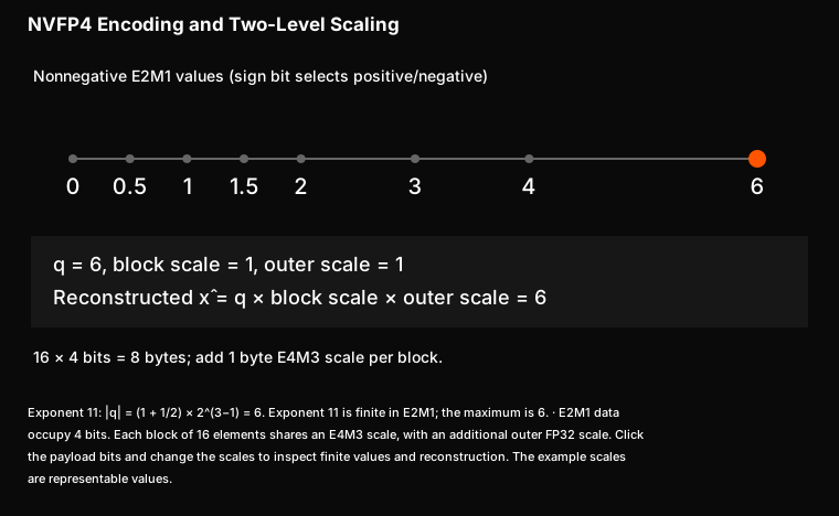
A Qwen3-0.6B NVFP4 pretraining checkpoint initially suffered severe performance degradation because its fused QKV structure was handled incorrectly. After the fix, mean Lambda accuracy was approximately 0.3043 for BF16, 0.3056 for one-dimensional quantization, and 0.3109 for two-dimensional block-scaled quantization. Conversion and structural adaptation must therefore be checked before attributing such a failure to the FP4 format.
For Qwen3-4B, online quantization reduced Lambda-base and Math23K scores by 0.0355 and 0.047 relative to BF16. Offline conversion introduced additional reductions of 0.0089 and 0.019. These comparisons separate the loss from the format and numerical path from the additional loss introduced by conversion and scale handling.
In RL, the two sides can differ substantially even when they use the same format. Early configurations produced the following mean absolute log-probability gaps:
| Training / sampling precision | Dense | MoE |
|---|---|---|
| BF16/BF16 | 0.0110 | 0.0172 |
| NVFP4/NVFP4 | 0.1142 | 0.0668 |
| NVFP4/BF16 | 0.1376 | 0.0621 |
| BF16/NVFP4 | 0.1690 | 0.0747 |
Table 1. Early training–sampling comparisons. The dense model is Qwen3-4B; the MoE model is Qwen3-30B-A3B. These results locate error sources within this set of configurations.
Replacing offline ModelOpt conversion with online quantization still left a gap of approximately 0.1142 for the dense model. Using the same quantization/GEMM operators on both sides also left residual differences. We therefore expanded the investigation to input organization, scale computation, and operations surrounding quantization.
2.3 Activation Precision, Scaling Granularity, and the KV Cache
With NVFP4 weights fixed, increasing activation precision tests the effect of activation quantization. W and A denote weights and activations; the following numbers give their bit widths, so W4A16 uses 4-bit weights and 16-bit activations:
| Weights / activations | Dense gap | MoE gap |
|---|---|---|
| W4A16 | 0.0139 | 0.0166 |
| W4A8, MXFP8 activations | 0.0363 | 0.0227 |
| W4A4, NVFP4 activations | 0.0903 | 0.0445 |
Table 2. Activation-precision comparisons using the corresponding unquant inference adaptation paths. This experiment and Table 1 belong to different stages of the investigation and are not a single ablation.
W4A16 brings the gap close to the BF16 reference, identifying activation quantization as an important factor in this configuration. In another fixed configuration, changing the KV cache from FP8 to BF16 reduces the gap from 0.0721 to 0.0583. Sampler-state precision also affects cross-framework agreement.
We next examine the scaling domain. Sampler decoding processes the current token, whereas the learner typically processes a full response at once. If the activation's outer scale uses tensor-wide amax, the same token can receive different scales depending on the other tokens in its batch. Per-token amax restricts the reduction domain to the current row and removes this dependency.
Let be a reference vector and its decoded approximation, each with elements. Relative L2 error is ; signal-to-noise ratio is , in dB; and mean absolute error is . The notation denotes the Euclidean norm. Relative error and SNR assume a nonzero reference vector. Lower relative L2 and MAE, or higher SNR, indicate closer reconstruction.
How the Scaling Domain Introduces Context Dependence
Interactive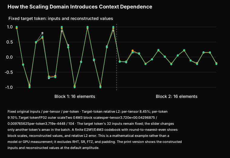
Scaling granularity does not determine all quantization error. We sweep exponent and mantissa widths on real QKV inputs. With E=2 and E4M3 scales fixed, increasing M from 1 to 4 raises mean SNR from 19.88 dB to 34.96 dB and reduces relative L2 from 0.10140 to 0.01807. Increasing exponent width does not always help and can interact poorly with the scale's representable range. These simulated formats identify sensitive factors; they are not additional hardware-native NVFP4 formats.
In one configuration, per-token amax changes the initial gap only slightly, from 0.05532 to 0.05501, while later runs show smoother training. This motivates examining error direction, local structure, and its evolution during training rather than relying on the initial average alone.
D1 · Exponent and Mantissa Sweeps: Real QKV Inputs, Simulations, and Initial RL Measurements
Real QKV Inputs: Varying Mantissa Width
| Format | SNR E4M3 | SNR E8M0 | Rel-L2 E4M3 | Rel-L2 E8M0 |
|---|---|---|---|---|
| E2M1 | 19.88 | 17.11 | 0.10140 | 0.13950 |
| E2M2 | 26.23 | 23.98 | 0.04885 | 0.06322 |
| E2M3 | 31.19 | 30.31 | 0.02767 | 0.03051 |
| E2M4 | 34.96 | 36.41 | 0.01807 | 0.01513 |
Table 2-1. QKV inputs collected from 36 layers during real prefill and single-token generation, summarized across layers. The simulated formats do not imply new hardware support.
Real Inputs: Exponent Range and Scale Range
| Data format | SNR with E4M3 (dB) | SNR with E8M0 (dB) |
|---|---|---|
| E2M1 | 19.88 | 17.11 |
| E3M1 | 21.50 | 19.7 |
| E4M1 | 14.39 | 19.7 |
| E5M1 | 0.0 (maximum exceeds E4M3 range) | 19.7 |
| Data format | Relative L2 with E4M3 | Relative L2 with E8M0 |
|---|---|---|
| E2M1 | 0.10140 | 0.13950 |
| E3M1 | 0.08478 | ~0.103 |
| E4M1 | 0.28937 | ~0.103 |
| E5M1 | 0.99698 (maximum exceeds E4M3 range) | ~0.103 |
E3M1/E4M1/E5M1 with E8M0 scales behave similarly over the measured input range. Combining E4M3 scales with a wider data range can create scale-range problems. More exponent bits therefore do not necessarily improve accuracy for these inputs.
Initial RL Gap: Exponent and Mantissa Width
| Data format | Initial gap with E4M3 |
|---|---|
| E2M1 | 0.05800700932741165 |
| E3M1 | 0.11516289412975311 |
| E4M1 | 3.412203073501587 |
| E5M1 | nan |
| Data format | Initial gap with E4M3 |
|---|---|
| E2M1 | 0.05800700932741165 |
| E2M2 | 0.042353976517915726 |
| E2M3 | 0.03562581539154053 |
| E2M4 | 0.031815189868211746 |
Table 2-2. Recorded initial gaps, including NaN outcomes. These measure initial agreement; long-run training is evaluated separately.
Simulated Inputs and Real-Input Comparisons
| Data format | Scale format | MAE | SNR dB |
|---|---|---|---|
| E5M1 | E4M3 | 1.485030 | 0.00 |
| E4M1 | E4M3 | 0.132963 | 20.48 |
| E3M1 | E4M3 | 0.127780 | 20.63 |
| E2M1 | E4M3 | 0.154619 | 19.62 |
| E5M1 | E8M0 | 0.128281 | 20.18 |
| E4M1 | E8M0 | 0.128281 | 20.18 |
| E3M1 | E8M0 | 0.128515 | 20.18 |
| E2M1 | E8M0 | 0.176643 | 17.97 |
| Data format | Scale format | MAE | SNR dB |
|---|---|---|---|
| E2M4 | E4M3 | 0.017888 | 36.91 |
| E2M3 | E4M3 | 0.034627 | 31.58 |
| E2M2 | E4M3 | 0.070138 | 26.04 |
| E2M1 | E4M3 | 0.142116 | 20.17 |
| E2M4 | E8M0 | 0.018970 | 37.03 |
| E2M3 | E8M0 | 0.038432 | 30.93 |
| E2M2 | E8M0 | 0.079777 | 24.93 |
| E2M1 | E8M0 | 0.176643 | 17.97 |
Table 2-3. MAE/SNR from two simulated input batches, corresponding to exponent and mantissa sweeps. They separate input-distribution effects from bit-width effects and are distinct from repeated measurements of real QKV means. The complete format summary follows.
| Format | Mean SNR | Worst SNR | Mean MAE | Mean relative L2 |
|---|---|---|---|---|
| E2M4 + E8M0 | 36.41 | 35.87 | 0.007954 | 0.01513 |
| E2M4 + E4M3 | 34.96 | 29.58 | 0.007589 | 0.01807 |
| E2M3 + E4M3 | 31.19 | 28.12 | 0.014404 | 0.02767 |
| E2M3 + E8M0 | 30.31 | 29.73 | 0.016283 | 0.03051 |
| E2M2 + E4M3 | 26.23 | 25.03 | 0.027865 | 0.04885 |
| E2M2 + E8M0 | 23.98 | 23.64 | 0.034200 | 0.06322 |
| E3M1 + E4M3 | 21.50 | 17.81 | 0.045411 | 0.08478 |
| E2M1 + E4M3 | 19.88 | 19.53 | 0.058788 | 0.10140 |
| E5M1/E4M1/E3M1 + E8M0 | ~19.7 | ~19.3 | ~0.051 | ~0.103 |
| E2M1 + E8M0 | 17.11 | 16.66 | 0.077184 | 0.13950 |
| E4M1 + E4M3 | 14.39 | 0.71 | 0.067209 | 0.28937 |
| E5M1 + E4M3 | 0.03 | 0.00 | 0.577118 | 0.99698 |
2.4 Mismatch Must Be Interpreted Alongside Update Direction
Let denote the advantage of response , measuring its reward relative to other responses in the same group. The figure abbreviates it as and writes a token’s gap as . In GRPO, a positive advantage tends to increase sampled-token probabilities; a negative advantage tends to decrease them. At synchronized weights, the gap reflects execution differences. After learner updates, it also includes parameter changes relative to the fixed sampling policy.
When the learner underestimates a token (δ < 0), a negative-advantage update lowers its probability further and can amplify the local discrepancy; a positive-advantage update tends to reduce it. The roles reverse when the learner overestimates the token (δ > 0).
Intervention therefore needs both gap magnitude and update direction. TRIAGE uses the signs of advantage and gap to identify local risk. This local analysis motivates the algorithm; actual updates also depend on cross-token coupling and the optimizer.
Update Direction Determines Local Mismatch Risk
Interactive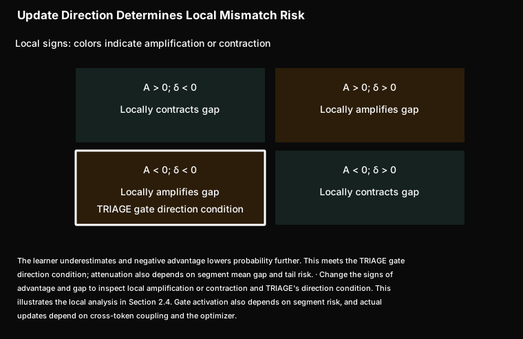
A > 0, δ < 0
The learner underestimates and positive advantage raises probability, locally approaching the sampler. TRIAGE repair separately acts on negative segments in positive-advantage responses.
A > 0, δ > 0
This can locally amplify mismatch. TRIAGE does not attenuate every amplifying quadrant: its gate direction condition is negative advantage and negative gap.
A < 0, δ < 0
The learner underestimates and negative advantage lowers probability further. This meets the TRIAGE gate direction condition; attenuation also depends on segment mean gap and tail risk.
A < 0, δ > 0
The learner overestimates and negative advantage lowers probability, locally approaching the sampler.
2.5 Averages Can Hide Local Risk
In one diagnostic trajectory for each model, directional changes precede the explosion of the global tail. When responses are divided into 64-token segments, a small fraction of tail-dense segments accounts for part of the severe mismatch. A response containing these segments can still have a small average gap.
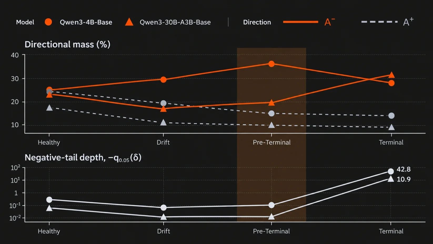
Experimental results
Figure 1. Directional distributions and negative tails from TRIAGE's supplementary analysis. The upper panels show region shares weighted by the original ; the lower panels show negative-tail depth, , where is the fifth percentile of the token gaps and is the absolute advantage. The 4B analysis uses direct gaps; the 30B analysis uses residual gaps after routing replay. Stage definitions and local thresholds are given in the appendix.
These findings create two needs: an algorithm to manage risky updates in existing stacks, and shared interfaces for comparing scales, precisions, and operator paths. We next introduce TRIAGE, then describe how miniTE brings alignment, experimentation, and efficient execution into a reusable framework.
Diagnosis · §2With NVFP4 weights fixed, W4A16 brings the gap close to the BF16 reference level; moving the KV cache from FP8 to BF16 reduces the gap from 0.0721 to 0.0583.
3. TRIAGE: Direction-Aware Stabilization of Native NVFP4 RL
3.1 Mechanism
TRIAGE operates on a policy objective that already includes importance corrections such as truncated importance sampling (TIS) [10]. It retains native NVFP4 forward computation and manages residual mismatch by modifying the optimization objective. The method combines segment diagnostics, a direction-selective gate, and bounded repair.
The gate uses mean gap and deep-tail token counts in 64-token segments to assess risk. In high-risk segments with negative advantage, it attenuates update weights only for negative-gap tokens; all other tokens retain their original weights. The weighted loss is then normalized within each response, redistributing update contributions.
Repair adds a signal for negative segment offsets in positive-advantage responses. It applies a one-sided pseudo-Huber penalty with bounded derivative to mean gaps in 128-token segments, increasing learner log probabilities in active segments. The gate reduces risky updates, while repair supplies a segment-level corrective signal. Parameters and normalization are specified in Appendix B.
3.2 Stability and Task Performance
TRIAGE's NVFP4 baselines already use per-token activation scaling on both sides. The experiment measures residual mismatch in that native stack. TRIAGE completes 600 training steps for 4B and 1,700 for 30B. TIS delays but does not prevent instability for 4B; for 30B, it completes training with weaker late-stage performance.
TRIAGE Training Dynamics
Interactive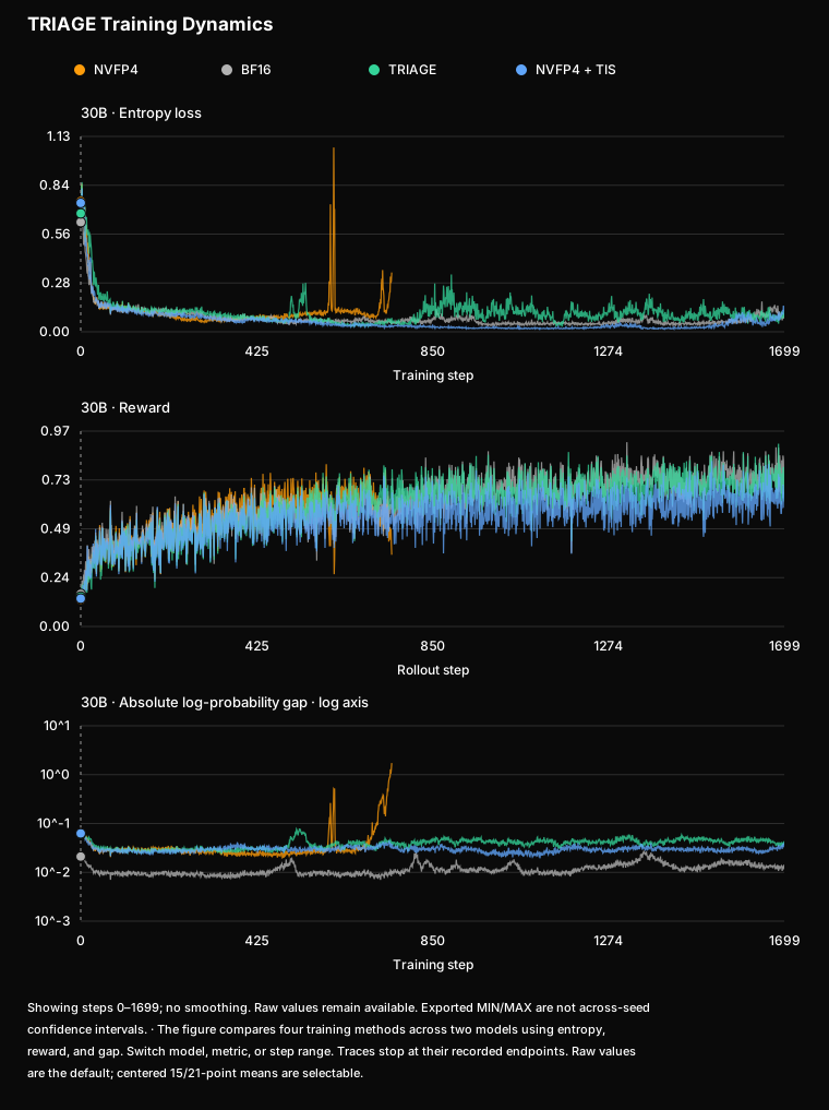
Figure 2. TRIAGE training dynamics. The upper row is 30B and the lower row 4B. From left to right: entropy loss, reward, and mean absolute gap.
| Configuration | 4B checkpoint | Five-math-task mean | 30B checkpoint | Five-math-task mean |
|---|---|---|---|---|
| BF16 | 600 | 58.26% | 1,700 | 72.41% |
| NVFP4 | 300† | 47.10% | 700† | 65.87% |
| NVFP4 + TIS | 300† | 50.76% | 1,700 | 63.18% |
| NVFP4 + TRIAGE | 600 | 58.49% | 1,700 | 70.96% |
Table 3. Unweighted mean over AIME24, AIME25, MATH-500, AMC23, and GSM8K [11,12,13]. † marks a checkpoint saved before instability. Final results with different training durations are distinguished from equal-budget comparisons.
At the shared 4B step-300 checkpoint, TRIAGE scores 53.03%, exceeding native NVFP4 and TIS by 5.93 and 2.27 percentage points. Its benefit therefore also appears at equal training budgets. Framework throughput is evaluated in the miniTE test environment.
3.3 Two Complementary Approaches
TRIAGE and miniTE intervene at different points in the problems identified above. TRIAGE changes updates when residual mismatch remains. miniTE directly examines and improves quantization, operators, and their invocation while reducing execution cost. The following sections introduce miniTE’s approach to numerical alignment and efficient computation. We evaluate the two approaches separately; additional gains from combining them remain to be tested.
4. miniTE: Aligning Numerical Execution and Optimizing Low-Precision Compute
4.1 Controlling Numerical Differences and Execution Cost
NVFP4 experiments repeatedly require local changes: activation-scale granularity, higher precision for selected layers, backward formats, and quantization or GEMM implementations. When these choices are tightly coupled to model modules, distributed communication, and training scripts, each experiment must also revisit surrounding logic, making errors harder to locate.
miniTE addresses these issues at the execution layer, making quantization rules explicit and comparing the learner and sampler at matching numerical boundaries. It provides ordinary linear layers, combined LayerNorm–linear modules, and MoE GroupedLinear modules. A common quantization interface connects Python references and optimized backends. Megatron and the upper-level RL system still orchestrate training, while inference frameworks such as SGLang perform sampling [7,8]. miniTE focuses on integrating, comparing, and optimizing numerical policies and operators.
miniTE Framework and Compute Paths
Interactive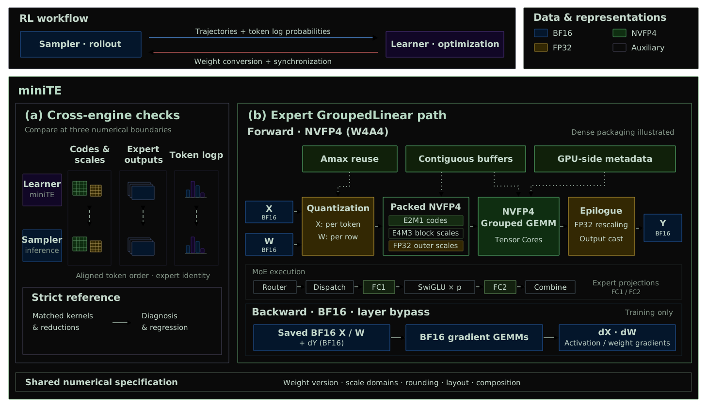
4.2 Layered Interfaces and Transformer Engine Integration
The module layer retains parameters, autograd, and distributed interfaces needed by the training framework. The quantization-policy layer specifies formats and scales. Compute backends implement quantization and GEMM. Developers can validate numerical behavior with a reference before integrating CUDA, CUTLASS, or TE implementations behind the same interfaces.
| Layer | Components | Extension point |
|---|---|---|
| Module | Linear, LayerNormLinear, GroupedLinear | Model integration and distributed wrappers |
| Precision configuration | RecipeSpec, get_qlinear_params, QLinearParams | Named selection; activation, weight, gradient, and fprop/dgrad/wgrad precision |
| Quantization interfaces | quantize, group_quantize | Quantization parameters, scale granularity, padding, grouping |
| Matrix multiplication | qgemm and backends | Encoded data, scale layouts, GEMM dispatch |
| Diagnostics | Tensor statistics, profiling, cross-framework collection and comparison | Numerical regression and profiling |
Table 4. miniTE responsibilities. New numerical policies are primarily implemented in the quantization and backend layers, reusing shared module logic.
TE integration is a core design requirement. miniTE follows existing Linear interfaces and checkpoint parameter names so Megatron wrappers can replace the corresponding modules while reusing the surrounding training workflow. Parameter loading, extra state, and parallel modes are validated for each integration path to balance migration cost and behavioral consistency.
The recipe registry stores names, purposes, and dependency metadata; the parameter factory converts the selection into QLinearParams. The registry and inspection entry points use only the Python standard library. Operator imports are deferred to the corresponding factory branches, so developers can inspect a configuration before preparing its CUDA, TE, and compiled dependencies. Reference and optimized paths continue to share the upper-level modules.
4.3 Precision Recipes and Selective Quantization
The W4A16, W4A8, and W4A4 experiments in Section 2 require independent configuration of weights and activations. miniTE additionally separates gradient precision and GEMM settings for forward propagation (fprop), input gradients (dgrad), and weight gradients (wgrad). A new forward quantization policy therefore need not commit to a particular backward precision.
Version 1.0.0 selects named recipes through MINITE_RECIPE or get_qlinear_params, including nvfp4_per_token and nvfp4_per_token_bf16_bwd. Explicit layer qlinear_params take priority over environment selectors. Layer-name overrides and layer-number quantization exclusions support sensitivity analysis. Development can begin with reference quantization: establish scales and encoding, choose a GEMM backend, then compare full-precision and quantized backward paths.
miniTE CUTLASS and miniTE per-token are two implementations of MoE GroupedLinear. Both use NVFP4 forward computation and compute activation outer scales per token. CUTLASS names a matrix-multiplication implementation, whereas per-token names a scaling granularity; the terms are not mutually exclusive, and the TE per-token path also calls CUTLASS kernels. The main differences are below.
| Property | miniTE CUTLASS | miniTE per-token |
|---|---|---|
| Activation outer scale | One per token | One per token |
| Weight outer scale | One per expert weight tensor | One per row of the flattened expert weights |
| Quantization and GEMM interfaces | miniTE packing and CUTLASS V2 grouped GEMM | TE per-token bulk quantization and grouped GEMM, with list/dense packaging |
| Recipe | nvfp4_cursor2_cutlass_v2 | nvfp4_per_token |
Both paths were tested with MXFP8 backward and BF16 backward. Backward precision is configured separately and cannot be inferred from the path name. The reported BF16-backward performance uses the layer bypass, which saves the original BF16 operands and skips backward quantization. The dedicated nvfp4_per_token_bf16_bwd operator is a separate implementation and requires its own performance measurements.
NVFP4 Forward with Independently Configured Backward Precision
Interactive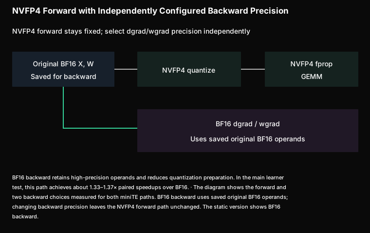
Public selectors resolve recipes through one registry, grouped by common, reference, and experimental use. These groups describe purpose. describe reports forward/backward behavior and requested layout; doctor checks the selected runtime prerequisites. Each result records forward and backward precision, quantization coverage, and source revision.
4.4 Numerical Monitoring, Profiling, and Alignment Diagnostics
Low-precision failures may emerge late in training. miniTE therefore provides configurable numerical and performance collection. Developers can inspect activation, weight, output, and gradient minima, maxima, means, and norms by module, instance, rank, and step, and save tensors to reproduce anomalies. The profiler produces Chrome traces and kernel timing statistics, separating computation, preparation, and gaps between calls.
Comparing the learner and sampler first requires aligning their inputs. MoE dispatch can change token order on the two sides; direct elementwise subtraction would then mistake permutation differences for numerical error. We collect routing information, expert FC1/FC2 tensors, and token log probabilities, align token and expert identities, and then compare outputs, quantized data, and scales.
Diagnostics distinguish actual kernel outputs, hook boundaries, and reference replay. Replay can locate an issue when an intermediate inside a fused kernel cannot be collected directly, but its provenance remains explicit. Agreement in replay is different from agreement in actual execution. Each recipe or kernel change can then be traced through inputs and routing, quantization, GEMM, and output probabilities.
4.5 Train–Inference Alignment and Deterministic Execution (Deterministic Mode)
Low-bit training stability depends on quantization precision and on whether operators behave consistently in training and inference. Even with the same quantization policy, small differences in operator implementations, reduction order, or parallel execution can accumulate into numerical discrepancies that affect training.
We therefore implement deterministic mode in miniTransformer: layer-by-layer replacement of Megatron operators makes them use the same kernels, formulas, and reduction order as SGLang inference. Multiple checked key layers achieve bit-exact agreement.
This layerwise alignment works with the tensor and routing-identity checks in Section 4.4. In the original record, TIS is disabled for the strict configuration and enabled for non-strict references. The figure therefore retains the joint identity of execution paths and algorithmic correction; bit-exact layer agreement and the end-to-end log-probability gap are reported separately.
NVFP4 Alignment and Training Stability
Interactive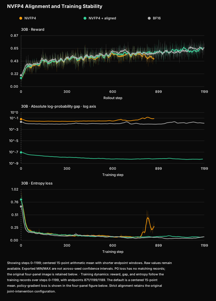
Reward, gap, entropy, and policy-gradient loss
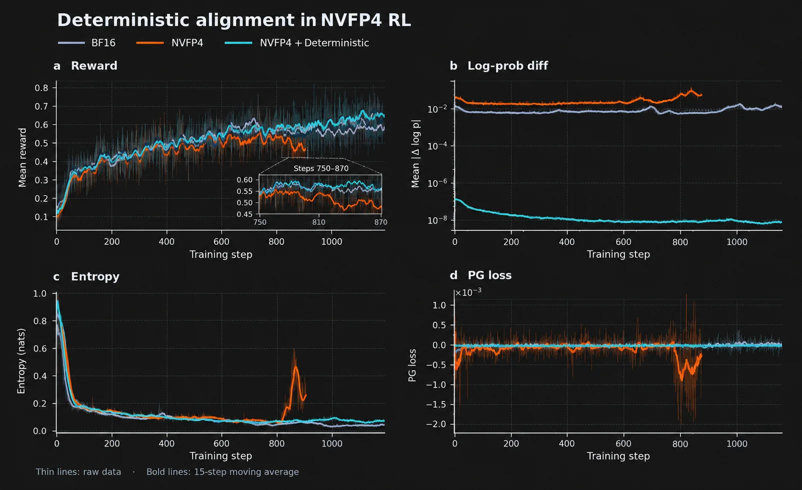
Figure 4. Training–sampling alignment: reward, mean absolute log-probability gap, entropy, and policy-gradient loss. Thick lines are 15-step moving averages. The aligned configuration reaches a gap of approximately over the measured interval and maintains relatively steady late-stage reward. Multiple implementation choices change together in this comparison.
In this experiment, the aligned train–inference log-probability difference falls to approximately , with steady late-stage reward and smaller perturbations. Unaligned NVFP4 shows a late reward decline accompanied by rising entropy and log-probability difference. Within this configuration, smaller train–inference discrepancies accompany steadier NVFP4 RL dynamics. This is a single-run comparison of different implementation configurations with multiple choices changing together. Alignment and throughput measurements also have separate experimental identities; performance remains based on direct measurements of the corresponding Section 6 configurations.
miniTE provides alignment capabilities together with the configuration, debugging, and extension interfaces needed to implement them. New low-precision policies can follow the same validation process from local correctness to RL training.
Alignment · §4.5Under the strictly aligned configuration, the train–inference log-probability gap stays around 10⁻⁸, with stable late-stage reward.
5. Joint NVFP4 Implementation and Optimization with Transformer Engine
5.1 Numerical and Implementation Choices for Per-Token Scaling
We conduct joint testing and implementation work with NVIDIA around TE's NVFP4 support, using the per-token recipe and its interfaces as an important integration point [9]. Scale granularity affects numerical behavior as well as amax computation, scale storage, and GEMM epilogue cost. Accuracy and speed therefore need to be evaluated together.
NVFP4 encodes data in E2M1, uses an E4M3 scale for each block of 16 elements, and adjusts the range with an outer FP32 scale [1]. Let be the outer scale of row , and its length-16 block. Then
Per-tensor scaling shares one outer scale across a tensor; per-token scaling computes it per row. The latter reduces dependence on other tokens' maxima and can mitigate block-scale underflow when row magnitudes differ greatly. It still retains within-row dynamic-range and FP4 rounding error, and requires finer-grained compute support. Public systems also combine per-token NVFP4 forward computation with higher-precision backward computation [2].
We retain multiple recipes and evaluate numerical choices separately from implementation optimizations. Lower local quantization error alone does not establish more stable RL training. The cost of additional reductions is likewise evaluated over the full computation path.
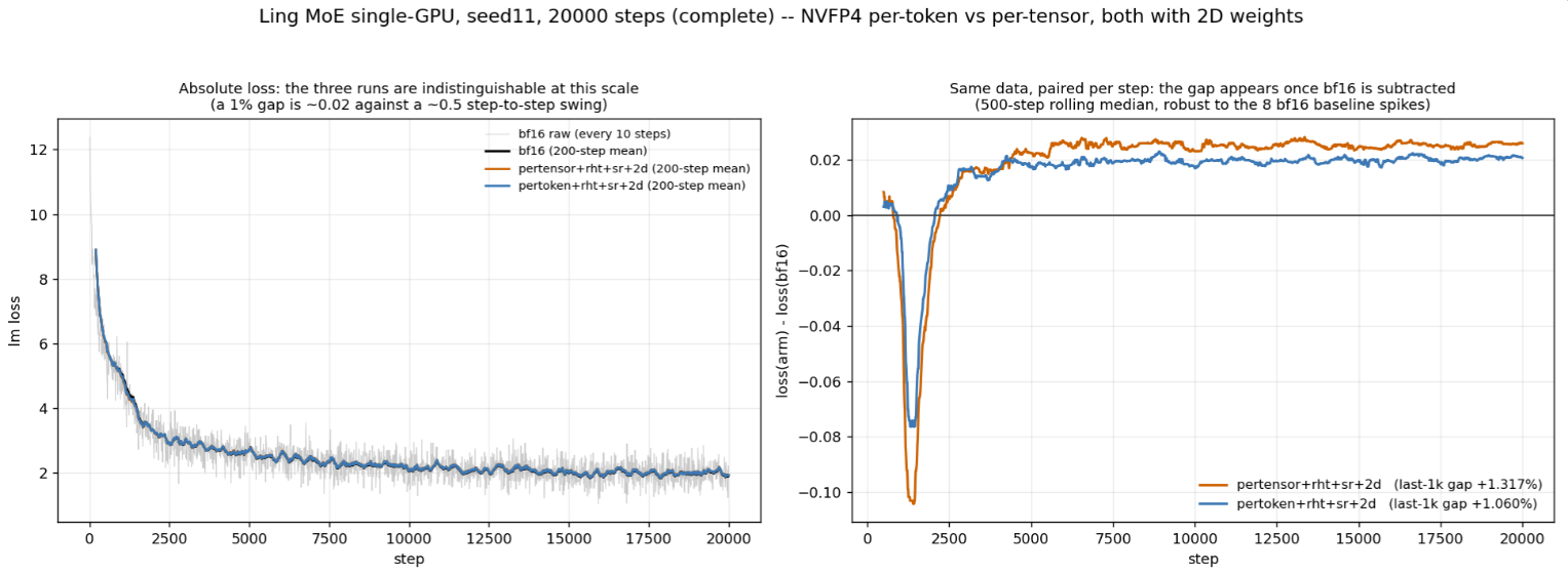
D2 · 20k-Step Language-Model Loss: Per-Token versus Per-Tensor Scaling
Experimental results
Figure 5-1. Ling MoE, single GPU, seed 11, 20,000 steps. Both NVFP4 configurations use RHT, SR, and 2D weight quantization. The left panel shows absolute loss; the right subtracts BF16 loss on the same data. Relative gaps over the final 1k steps are per-tensor +1.317% and per-token +1.060%.
Absolute losses are close at the plotted scale; subtraction from BF16 reveals the smaller differences. This supplies long-run language-model loss evidence for the scaling choice. It is distinct from the RL+TIS trajectories in Section 6.2.2 and does not independently establish RL stability.
5.2 Contiguous Layouts and Grouped GEMM Invocation
Original grouped interfaces may split quantized data and scales into separate expert tensors, then reconstruct pointers, strides, and layouts for GEMM. As expert counts increase, Python/ATen slicing, list construction, temporary allocation, and host-to-device metadata transfers can offset FP4 arithmetic gains.
We organize quantization outputs into contiguous buffers and describe expert boundaries with offsets, passing them directly to dense grouped GEMM. FP4 data, block scales, and outer scales travel through the same interface, avoiding splitting after quantization and reassembly before computation. Device-side metadata construction and workspace reuse reduce allocation and synchronous copies. Zero-token experts and padding are handled within the same grouped path.
This optimization changes data organization and invocation. Dense quantization and GEMM interfaces are checked against the original list path for operands and outputs; performance is measured for the combined implementation. Revision b641179 later combines the dense path, GEMM settings, and fusion. The core repeated tests retain their original revision identity.
5.3 Computing amax Where Data Are Produced
A separate amax kernel first scans activations, after which the quantizer reads them again. We look for operations that already traverse the data along the producer-to-consumer path.
For MoE FC1, inputs pass through dispatch and permutation, allowing rowwise amax to be accumulated during token reordering. Padding processes activations and amax together, so quantization can reuse the external statistics and skip repeated reduction.
For MoE FC2, amax is better fused with activation computation. We use _weighted_swiglu_row_amax_kernel as the fused kernel, following the JIT-compiled implementation and accumulating amax while traversing columns. The statistic applies to the SwiGLU output after router weighting, exactly the tensor passed to FC2 quantization. Reusing the existing memory and computation path avoids another complete scan of the FC2 input for amax.
The FC1 transformation is:
Original: sort → pad(activation) → amax → quantization
Fused:    sort + amax → pad(activation, amax) → quantization
FC2 produces amax together with weighted activations and reuses it in subsequent quantization:
Original: SwiGLU × router weight → activation → amax → quantization
Fused:    weighted SwiGLU + row-amax → activation, amax → quantization
The benefit must cover the producer, padding, and consumer. Module-level simulations that skip amax are not always faster, so eliminating one kernel does not by itself establish a complete-flow benefit. Section 6 uses learner timings that include surrounding work.
5.4 Kernel Optimizations and Their Scope
Kernel-level optimization addresses cross-CTA amax reduction, FC1/FC2 GEMM pipelines, scale-layout transfer, and activation/amax fusion in the epilogue. The implementation details and applicable scope follow.
Expand: Kernel-Level Implementation Details
1. Row-amax: cluster shared memory for cross-CTA reduction. The K1 stage of per-token NVFP4 reduces amax across K-tiles for every row. The original path combines tile results with atomicMax. In the optimized path, CTAs first compute partial amax and write to the leader CTA's shared buffer. The leader reduces within the cluster. A cluster covering all K-tiles directly produces final row-amax; larger ranges fall back to atomics. In the recorded tests, n_cluster=16 and k_tile=128 cover K=2048, while increasing the tile to 256 covers K=4096. This replaces only K1 amax; K2 cast remains separate. The multi-cluster scheme showed no benefit and was removed. The optimization applies where a single cluster covers all or most of K, without extrapolating its benefit to larger K.
2. FC1/FC2 GEMM: choose tiles and pipelines by reduction length. Both layers use grouped NVFP4 GEMM, but their K lengths and epilogue-overlap conditions differ. FC1 has a longer K and MMA loop. MMA_N=256 with 2SM increases work per CTA and gives epilogue work more opportunity to overlap MMA. FC2 has a shorter K; reusing 256 columns with OverlappingAccum can make epilogue reads compete with MMA writes for the next stage. It therefore uses MMA_N=128 and 2SM. TMEM has 512 columns. A two-stage 256-column tile fills that capacity, leaving no room for scales and requiring an OverlappingAccum strategy instead of default TMEM allocation. These are configurations for the tested FC1/FC2 shapes; the optimal choice varies with shape.
3. Fused swizzle: write the GEMM scale layout directly during cast. Downstream GEMM requires a specific swizzled scale-factor layout. The original implementation produces compact M-major scales, then launches nvte_swizzle_scaling_factors, adding a kernel launch and global-memory traffic. The fused implementation adds a with_swizzle path to launch_grouped_fused_cast_bf16, writing the cuBLASLt 128M × 4K tile layout directly in DO_ROW. When disabled, the compact layout and separate conversion remain available. This eliminates intermediate scale reordering while retaining the quantization formula. Subsequent miniTE per-token tests found bit-exact agreement in quantized payloads, scales restored to the same layout, and final outputs between fused and unfused paths.
4. Activation and epilogue fusion: compute gating and statistics at the FC1 output. MoE FC1 produces paired gate/up tensors, usually followed by SwiGLU or GeGLU and output-side amax for subsequent quantization. The fused epilogue performs alpha/bias correction, paired gate/up activation, router-probability weighting, and D-side amax. Depending on the configuration, it preserves optional writes of the pre-GLU intermediate C; the FP8 path can also generate output scale factors. The core dataflow is:
ACC = block-scaled GEMM(A, B)
ACC = ACC × α_a[m] (optionally × α_b[n]) + bias
C = gate | up (pre-GLU, width N; optionally written)
D = act(gate, up) × prob (SwiGLU/GeGLU, width N/2)
Reduce D amax concurrently; FP8 can generate output scale factors
Computing activation and statistics in place reduces writes and subsequent reads of complete gate/up intermediates, together with separate activation/amax kernel launches. This fusion currently targets forward paths in which FC1 immediately feeds gated activation and quantization statistics. Inclusion in the main performance configuration is recorded separately for each optimization; complete benefits remain based on the corresponding module and learner timings.
5.5 How Joint Testing Informs Implementation Choices
Joint work follows reference implementation, optimized implementation, module comparison, and model testing. Comparisons at a fixed recipe validate interface and layout changes; comparisons across recipes evaluate precision choices and their costs. BF16, native TE NVFP4, our CUTLASS path, and the upstream per-token implementation serve different baseline roles.
This process integrates TE capabilities into miniTE and brings bottlenecks found in miniTE back to TE interfaces and kernels. Public per-token implementation and discussion are available in PR #3045 [9]. Revisions, patches, and test scope accompany the results; attribution and upstream merge status follow the actual records.
5.6 Exploring Single-Pass Fusion
We also investigate online amax compensation for fused SwiGLU-FFN paths that avoid materializing the full intermediate activation. FC2 consumes activation K-tiles before the full-row amax is known. The method maintains a running rowwise amax and converts earlier partial accumulations to the new scale whenever the outer scale increases, connecting FC1, SwiGLU, quantization, and FC2.
This path primarily reduces intermediate-activation memory traffic and separate kernel calls. Compensation maintains a consistent scale when accumulating tile contributions; the E4M3 block scales and E2M1 codes produced earlier still depend on the scale and rounding used at that time. We therefore retain it as a fusion research direction, evaluating compensation error, quantization differences from two-pass execution, and the complete call-chain benefit separately.
Expand Online Amax Compensation Quantization
Algorithm: accumulate FC2 partial outputs in the current row scale
Let denote the SwiGLU activation for FC2 K-tile . Complete the FC1 reduction for the corresponding gate/up slice, then compute SwiGLU, the rowwise absolute maximum, and the maximum of each 16-element block. The running rowwise amax and outer scale are
For block , the quantizer produces and . FC2 block-scaled MMA computes
Here, includes the weight block scales but excludes the outer weight scale , which is constant along K. The rowwise activation scale and outer weight scale are broadcast over their corresponding output dimensions. If the outer weight scale varies by tile, incorporate that variation into each partial instead of applying one common factor at the end. Activation bs is applied block by block inside MMA; only the outer gs is deferred to the epilogue.
Numerical conditions: avoiding saturation does not imply invariance for every gs
For fixed data, keeps the unrounded block scale within the E4M3 maximum of 448. The online running amax covers the current tile maximum, so the current tile satisfies this condition against upper-range saturation.
Without E4M3 rounding, , allowing the block scale to cancel an outer-scale change. In practice, rounded bs leaves a scale-dependent rounding residual in this product; a large gs may also push small blocks into the subnormal or underflow range. Power-of-two rescaling can preserve the decoded step size when the codebook stays in the normal range, avoids its boundaries, and uses consistent rounding. Arbitrary scale ratios do not have this guarantee.
The original heavy-tailed example uses one activation row with amax approximately 29. The design scale and four times that scale both yield rel-L2 0.099; reducing the scale to one quarter of the design value raises rel-L2 to 0.52:
| Outer scale | rel-L2 | Block-scale upper-range behavior |
|---|---|---|
| amax / 2688 | 0.099 | 1/16 reaches 448 exactly, without exceeding it |
| 4 × amax / 2688 | 0.099 | No block reaches the upper limit |
| amax / (4 × 2688) | 0.52 | 6/16 exceeds the upper limit and is clipped |
This example illustrates the role of the saturation condition and equal error under the specified scale multiplier. It does not establish identical codes or errors for every scale above the lower bound.
Compensation: merge partials in one common outer scale
has not yet been multiplied by its tile's , so partials from differently scaled tiles cannot be added directly. The recurrence converts the old accumulator to the current scale. Expanding it in ideal real arithmetic gives
The identity restores the outer scale of each already-quantized tile. It does not recompute earlier bs or q, and therefore does not establish bitwise equivalence to two-pass quantization with a known full-row amax. FP32 ratios, multiplication, and accumulation also round and must be checked in numerical comparisons.
The original diagnostic uses two slices with amax 1 and 100 and an FP32 reference. Directly adding differently scaled partials yields rel-L2 2618%. Restoring each slice's scale before summation and using sequential ratio compensation both yield a recorded rel-L2 of 6.0%, within the quantization-error range of this example.
| Merge method | rel-L2 (%) | Interpretation |
|---|---|---|
| Add both partials directly | 2618 | Mix outputs represented in different outer scales |
| Restore each gs, then add | 6.0 | Restore each tile's actual contribution |
| Running-scale ratio compensation, then restore gs | 6.0 | Perform the same scale conversion recursively |
Implementation flow and overhead
The fusion prototype targets SM100 (Blackwell) through CuTeDSL. FC1 accumulates the corresponding gate/up slice in TMEM, then transfers it to registers for SwiGLU, absolute rowmax, and quantization, with running amax stored in a workspace. FC2 directly consumes E2M1 data and E4M3 block scales. Its epilogue retrieves partials from TMEM and compensates and merges them in registers or SMEM. The core flow in the normal numerical range is:
Inputs: X, W_FC1, W_FC2
Initialize gamax = 0, gs_prev = 0, O = 0
for each FC2 K-tile i:
    Complete FC1 reduction for gate/up slice → SwiGLU → P_i
    rowmax = max(|P_i|); gamax = max(gamax, rowmax)
    If gamax = 0: this row contributes zero; skip computation
    gs = gamax / 2688
    Generate E4M3 bs and E2M1 q per 16-element block
    FC2 block-scaled MMA → ΔO_i (includes block scales, excludes gs)
    O = O × (gs_prev / gs) + ΔO_i
    gs_prev = gs
Y = O × gs_prev × gs_W2; all-zero rows output zero
SwiGLU outputs can be negative, so rowmax must use max(|P|). Explicitly set q=0 for all-zero rows or blocks to avoid 0/0. If a nonzero block's scale underflows, apply the quantizer's zero-value rule and record the associated error.
This path avoids writing and reading the full FP32 intermediate activation, but O must remain outside TMEM, adding partial transfers and a merge for every K-tile. In the supplied B200 Qwen3-30B-A3B shape-test record, the prototype is 4–8× faster than the unfused TE two-level chain, with accuracy close to that path. Against the fused single-level path, merge overhead is more visible for a 512-token small batch, while the gap at 4096 tokens is approximately 5%. Prefill and larger batches are therefore useful workloads for further evaluation. This prototype shape test is measured separately from the complete B300 learner tests in Section 6.
6. Evaluation: Numerical Correctness, Learning, and Execution Efficiency
We validate the preceding implementation choices by checking quantization, interfaces, matrix multiplication, and gradients, then evaluating long-run learning. We next measure complete learner updates, modules, serving, and online RL stages. Each experiment reports its result and how it informs implementation choices.
The main text presents key trends and results. Complete shape, gradient, repeated-run, and configuration data accompany the corresponding sections. The web reader provides these under their titles; printing collects them in Appendix C.
6.1 Setup and Measurement Scope
This section evaluates miniTE system performance; Section 3 reports TRIAGE's algorithmic results. The main performance model is Qwen3-30B-A3B on one node with 8×B300 and TP/PP/CP/EP = 1/1/1/4. Learner tests use sequence length 4096, micro-batch size 1, and GBS 128, processing 524,288 tokens per update from the same checkpoint, seed, and frozen DAPO text. Module, learner, serving, and online RL tests have distinct timing scopes.
| Experiment | Question | Measurement scope |
|---|---|---|
| Quantization / API / GEMM / gradients | Does optimization alter numerics? Where does error arise? | Reference kernel or FP32 golden; matching inputs |
| Long-run training and task evaluation | Does the configuration sustain effective learning? | Training trajectories and checkpoint evaluations |
| Module forward / direct F+B | Where are local gains and backward costs? | Quantization and expert GEMM; dispatch excluded |
| Fixed-text learner update | Do local optimizations improve complete updates? | Forward, backward, communication, optimizer, data loading |
| Fixed-output serving | How much does sampling capacity improve? | Eight-engine output throughput; learner and sync excluded |
| Online RL stages | Which system costs offset compute gains? | Logprob + actor train and conversion/sync measured separately |
D3 · Configurations, Forward and Backward Precision, and Statistical Units
| Configuration | Forward path | Backward / coverage | Role |
|---|---|---|---|
| TE BF16 | TE BF16 GroupedLinear | BF16 | High-precision reference and baseline |
| TE NVFP4 | Native TE per-tensor NVFP4 | Tested native recipe; non-expert layers BF16 | Existing NVFP4 path |
| miniTE CUTLASS | Custom CUTLASS NVFP4 | MXFP8 and BF16 backward tested separately | Custom path and precision choice |
| miniTE per-token | Per-token NVFP4 based on PR #3045 | MXFP8 and BF16 backward; expert-only | Per-token path and optimization chain |
| TE per-token | Fixed upstream per-token implementation | Same module-forward recipe; full-model coverage/backward documented separately | Module implementation and configuration timing reference |
Table 6-1. Comparison identities. Both miniTE paths are tested with MXFP8 and BF16 backward; the main learner configurations use BF16 backward.
- Module tests use five independent processes, taking the median within steady-state blocks for each run. The 4k/16k/64k/128k sizes denote pre-dispatch tokens per rank.
- Core learner tests use ten independent runs of 20 updates, with the first five as warmup and updates 6–15 measured. Throughput and paired speedups each discard their own minimum and maximum before averaging.
- The complete optimization chain uses one process per configuration and 17 updates. After two warmup updates, the minimum and maximum of 15 measured update times are removed; throughput is computed from the mean of the remaining 13 times. These updates belong to one process.
- The core revision is miniTE 953f17f9; the optimization run uses b641179 with the dense path, GEMM-kind, and fusion. TE's zero-token-expert update and interference in run 3 are described in Appendix A.3.
6.2 Correctness and Learning Behavior
6.2.1 Separate Checks for Quantization, APIs, GEMM, and Gradients
We validate local numerical boundaries before full training. API and layout optimizations compare encoding, scales, and outputs at a fixed recipe. Quantized computation is compared with FP32 references after dequantization. Backward tests check direction, magnitude, and signs against FP32 gradients under straight-through estimator (STE) semantics. This distinguishes format error from error introduced by an optimization.
miniTE per-token dense quantization and grouped GEMM pass 28/28 bitwise equivalence checks. Fused layouts add no discrepancy in seven synthetic and real-activation cases. For the tested configurations, these layout changes preserve the quantization results.
D4 · Eight Operator Paths and Their References
| Category | Operator / path | Test target | Reference / criterion |
|---|---|---|---|
| miniTE CUTLASS | group_quantize_nvfp4_pertoken_swizzled | Per-token NVFP4 activation quantization | Bit-exact against per-group reference; dequantization follows FP4/E4M3 scale semantics |
| miniTE CUTLASS | group_quantize_nvfp4_tensor_global_packed | Per-tensor/global NVFP4 weight packing | FP4 data and swizzled scales match per-expert quantize_weight_nvfp4_swizzled |
| miniTE CUTLASS | grouped_cutlass_gemm_v2 / v2_evt | FP4 grouped GEMM | FP32 GEMM golden after dequantization |
| CUTLASS end-to-end | miniTE CUTLASS GroupedLinear | Module forward and backward | Pure BF16 grouped matmul / FP32 golden gradients |
| miniTE per-token | nvfp4_per_token_group_quantize_bulk_dense | TE per-token group quant dense API | PR#3045 list API; bitwise identical |
| miniTE per-token | nvfp4_cutlass_grouped_per_token_gemm_dense | TE per-token grouped GEMM dense API | PR#3045 list API; bitwise identical |
| miniTE per-token | fused swizzle / unfused swizzle | Does scale-layout fusion add numerical error? | Fused and unfused end-to-end bit-exact |
| Both miniTE backward paths | dgrad / wgrad | Backward-gradient correctness | FP32 golden gradients; expected cosine > 0.99 under STE semantics |
Table 6-2. Objects and references used in correctness checks.
D5 · Extreme Inputs, Subnormals, and Scale Underflow
| Test | Result | Notes |
|---|---|---|
| CUTLASS activation quantization and weight packing | 50 passed | Includes 16 new extreme cases; 8 benchmark cases deselected |
| per-token dense quantization: extreme inputs | 8 passed | Extreme inputs for miniTE per-token dense quantization |
| CUTLASS weight-layout argument regression | 8 passed | Existing bit-exact regressions unaffected |
Table 6-3. Engineering regression tests for extreme inputs. Passed-test counts describe case coverage rather than model-training stability or statistical significance.
- Per-token activation quantization: FP4 data and scales match the per-group reference bitwise. Extreme magnitudes, values near the BF16 maximum, subnormals, and mixed-magnitude inputs produce no NaN/Inf. Global scales for subnormal rows can flush to zero.
- Per-tensor/global weight packing: Encoding and swizzled scales match the per-expert reference. A subnormal expert retains inputs around 9e-41 with relative L2 around 1.56e-2. Global-scale checks use a 3% relative tolerance rather than bitwise equality for every floating-point scale.
- miniTE per-token dense per-token quantization: q_row, block scales, and row_amax match the upstream list path. Very small rows can become zero through block decode-scale underflow. The tested production path requires m_splits to be multiples of 128.
These distinct zeroing and scale behaviors help distinguish format range, floating-point FTZ, and interface issues.
FP32 epilogues also have direct numerical support. Both ordinary miniTE CUTLASS grouped GEMM and the EVT path are compared with the FP32 golden reference after dequantization:
| Kernel | cosine | max_abs | norm_rmse |
|---|---|---|---|
grouped_cutlass_gemm_v2 | ≥ 0.999994 | ≤ 0.0156 | ≤ 0.0033 |
grouped_cutlass_gemm_v2_evt | ≥ 0.999999 | ≤ 0.0078 | ≤ 4e-5 |
Table 6-4. miniTE CUTLASS GEMM accuracy. EVT reduces the norm_rmse bound from approximately 0.0033 to the 4e-5 range, supporting a high-precision epilogue in this path.
Against pure BF16 forward computation, GroupedLinear has cosine similarity around 0.99095 and norm_rmse around 0.135, substantially larger than GEMM error against its own dequantized reference. The former includes information lost to FP4; the latter checks GEMM implementation. The reference determines what the accuracy metric measures.
BF16 backward dgrad/wgrad closely match the BF16 reference, with maximum relative L2 approximately 0.001663. MXFP8 backward has relative L2 approximately 0.03765 and sign agreement around 98.8%. This supports independently selecting backward precision in Section 4; Section 6.4 measures its execution cost.
D6 · Complete Gradient Results for Both miniTE Paths: Cosine, Relative L2, Sign Agreement, and Expert Metrics
| Backend | Backward path | dgrad cosine (min) | dgrad rel-L2 (max) | dgrad sign agreement (min) | wgrad cosine (min) | wgrad rel-L2 (max) | wgrad sign agreement (min) | Expert cosine (min) |
|---|---|---|---|---|---|---|---|---|
| miniTE CUTLASS | MXFP8 bwdquant | 0.999292 | 0.037626 | 98.802% | 0.999291 | 0.037653 | 98.802% | 0.999287 |
| miniTE per-token | MXFP8 bwdquant | 0.999292 | 0.037626 | 98.802% | 0.999291 | 0.037653 | 98.802% | 0.999287 |
| miniTE CUTLASS | BF16 backward | 0.999999 | 0.001660 | 100.000% | 0.999999 | 0.001663 | 100.000% | 0.999998 |
| miniTE per-token | BF16 backward | 0.999999 | 0.001660 | 100.000% | 0.999999 | 0.001663 | 100.000% | 0.999998 |
| BF16 PyTorch reference | BF16 matmul | 0.999999 | 0.001660 | 100.000% | 0.999999 | 0.001663 | 100.000% | 0.999998 |
Table 6-5. Worst-case gradient metrics across seeds and shapes. The reference computes and in FP32. A 100% sign-agreement rate does not imply bitwise FP32 equality.
D7 · Dense APIs and Fused versus Unfused Scale Layouts
| Test object | Shape coverage | Result |
|---|---|---|
nvfp4_per_token_group_quantize_bulk_dense | Small, 8 experts, 32 experts, extreme inputs | q / scale / amax all bitwise identical |
nvfp4_cutlass_grouped_per_token_gemm_dense | small, fc1-ish, fc2-ish | GEMM output bitwise identical, max_abs = 0 |
Table 6-6. Shape coverage and results for the dense interfaces.
| Case | fused vs unfused Rel-L2 | cosine | max_abs | FP4 data mismatch | Scale mismatch |
|---|---|---|---|---|---|
| Synthetic, multiple seeds / token counts | 0 | 1.0 | 0 | 0 / 96 groups | 0 / 96 groups |
| real dump | 0 | 1.0 | 0 | 0 / 12 groups | 0 / 12 groups |
Table 6-7. Differences in fused/unfused outputs and intermediates. The production miniTE per-token path has different shape constraints from earlier experimental paths; this table reports the production-path checks.
6.2.2 Supplementary Long-Run Learning Evaluation
Figure 5 compares BF16+TIS, native NVFP4+TIS, and miniTE+TIS. miniTE maintains reward growth during the first 1,000 steps and exceeds native NVFP4 later in the run; BF16 achieves higher reward over this interval. The two NVFP4 configurations have similar mean log-probability gaps but different learning trajectories. Average gap alone is therefore not a substitute for task performance.
Training Curves for the Practical miniTE Path
Interactive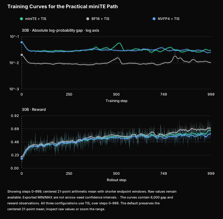
Figure 5. Learning dynamics of the practical miniTE path and baselines. Each configuration has one run over steps 0–999. The left panel shows mean absolute log-probability gap; the right shows reward. Thin lines are raw values, thick lines centered 21-step means. All configurations use TIS. This is a separate experiment from the strict alignment reference.
This supplementary run uses Qwen3-30B-A3B-Base. BF16, native TE NVFP4, and miniTE all use TIS, with routing replay disabled. Table 6-8 evaluates four mathematics tasks and IFEval on the respective step-999 checkpoints [11,12,13,14]. Each AIME benchmark averages six evaluations; MATH-500, GSM8K, and IFEval each average four. IFEval uses Prompt-level Strict accuracy. The BF16 checkpoint is evaluated with BF16 inference, and both NVFP4 checkpoints with NVFP4 inference.
| Configuration | AIME24 | AIME25 | MATH-500 | GSM8K | IFEval | Five-task mean |
|---|---|---|---|---|---|---|
| BF16 + TIS | 41.11% | 31.11% | 90.05% | 93.57% | 38.36% | 58.84% |
| TE NVFP4 + TIS | 26.67% | 20.56% | 86.90% | 94.71% | 43.99% | 54.57% |
| miniTE + TIS | 36.67% | 24.44% | 87.45% | 94.79% | 38.40% | 56.35% |
| miniTE minus TE NVFP4 | +10.00 | +3.88 | +0.55 | +0.08 | −5.59 | +1.78 |
Table 6-8. Task scores at step 999 of the supplementary run. The last row reports percentage-point differences. The five tasks receive equal weight, independent of evaluation counts. Repeated evaluation of a checkpoint does not create independent training seeds.
miniTE improves all four mathematics scores over native NVFP4. Its five-task average increases by 1.78 percentage points and remains 2.49 points below BF16. IFEval has a different ordering: miniTE is close to BF16 but below native NVFP4. These results support improvements on the measured mathematics training tasks, with downstream gains varying by task.
This supplements the framework's long-run training evaluation. Its task set, training duration, and evaluation protocol differ from TRIAGE in Section 3; each describes learning under its own configuration.
6.3 Complete Learner Updates: Do Local Changes Reduce Update Cost?
Table 6-9 summarizes the ten-run main test, comparing BF16, native TE NVFP4, and miniTE. Results for both miniTE paths also show how backward precision affects complete learner-update throughput.
| Configuration | Tokens/s, ten-run trimmed mean | Paired speedup over BF16 |
|---|---|---|
| TE BF16 | 24,192 | 1.000× |
| TE NVFP4 | 23,294 | 0.959× |
| miniTE CUTLASS, MXFP8 backward | 27,607 | 1.148× |
| miniTE CUTLASS, BF16 backward | 33,140 | 1.369× |
| miniTE per-token, BF16 backward | 32,517 | 1.334× |
Table 6-9. Complete learner throughput. Speedups are computed by pairing runs before trimming. Timing includes forward, backward, communication, the optimizer, and data loading; it excludes rollout and weight synchronization.
Complete Learner Throughput Across Repeated Runs
Interactive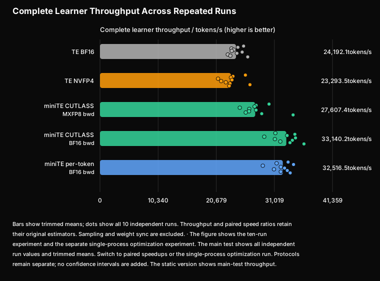
Both miniTE paths with BF16 backward achieve approximately 1.33–1.37× BF16 speed, while TE NVFP4 is near BF16. Moving miniTE CUTLASS backward from MXFP8 to BF16 further improves throughput, showing that lower-bit GEMM gains can be offset by backward quantization and preparation. miniTE per-token's ratio of aggregate throughput means against TE NVFP4 is approximately 1.396×. The 1.344× miniTE per-token/TE BF16 value is also a ratio of means, distinct from the 1.334× paired estimator here.
D8 · Ten Independent Runs, Trimmed Statistics, and Run Differences
| Run | TE BF16 | TE NVFP4 | miniTE CUTLASS MXFP8 backward | miniTE CUTLASS BF16 backward | miniTE per-token BF16 backward |
|---|---|---|---|---|---|
| 0 | 25545.3 | 25863.2 | 30070.0 | 31196.6 | 33463.5 |
| 1 | 24530.5 | 23653.1 | 27773.2 | 34662.4 | 31416.6 |
| 2 | 23384.9 | 23291.4 | 27501.7 | 33288.5 | 34428.9 |
| 3 | 23802.7 | 20997.8 | 24865.7 | 29218.7 | 28959.3 |
| 4 | 23437.2 | 23473.3 | 26551.5 | 34777.1 | 32164.2 |
| 5 | 25292.7 | 21553.5 | 27759.3 | 31109.0 | 32828.9 |
| 6 | 24352.1 | 22381.7 | 26508.3 | 34214.7 | 30948.3 |
| 7 | 22730.2 | 23138.2 | 25925.8 | 32078.5 | 33315.1 |
| 8 | 23191.5 | 26672.6 | 28769.0 | 33794.5 | 32159.6 |
| 9 | 26277.9 | 22993.5 | 34352.4 | 36279.4 | 33835.6 |
| Trimmed mean | 24192.1 | 23293.5 | 27607.4 | 33140.2 | 32516.5 |
Table 6-10. Throughput for every run in the machine-readable results, shown to one decimal place. Main-text summaries use integers.
An idle serving process occupied resources during run 3. The minimum observations for its quantized variants are removed by the predefined trimming rule. Early and later TE revisions handle zero-token experts differently; corresponding checks cover nonempty groups. Configurations are paired by run ID rather than simultaneous execution. A trimmed mean of paired speedups and a ratio of aggregate means are distinct estimators.
Data: ten-run records; runs and revisions.
D9 · Early Three-Run Results and Reserved Memory
| Configuration | Early-run tokens/s | Peak reserved memory (original MB) |
|---|---|---|
| TE BF16 | 25,545 / 24,531 / 23,385 | 119,914 |
| TE NVFP4 | 25,863 / 23,653 / 23,291 | 122,672 |
| miniTE CUTLASS MXFP8 backward | 30,070 / 27,773 / 27,502 | 144,598 |
| miniTE CUTLASS BF16 backward | 31,197 / 34,662 / 33,289 | 137,778 |
| miniTE per-token MXFP8 backward | 27,493 (run 0 only) | 138,458 |
| miniTE per-token BF16 backward | 33,464 / 31,417 / 34,429 | 133,398 |
Table 6-11. Early runs and peak reserved memory, retaining the original MB units. These are separate from later measurements in GiB under other protocols. miniTE per-token with MXFP8 backward has one reference run.
miniTE per-token reduces reserved memory relative to some miniTE variants but remains above BF16 in this comparison. Saved high-precision operands, quantized weight caches, workspaces, and padding all contribute to total usage; FP4 payload width alone does not determine model memory consumption.
The subsequent complete optimization chain combines the dense path, GEMM-kind, permutation fusion, and amax reuse. miniTE per-token with BF16 backward reaches 33,540 tokens/s, or 1.39× the same-round BF16 baseline and 1.47× TE NVFP4. This combined test uses a different revision and protocol:
D10 · Complete Fusion Run: Configurations and Timing Protocol
| Configuration | Fusion-run tokens/s | Speedup over same-round BF16 |
|---|---|---|
| TE BF16 | 24,134 | 1.000× |
| TE NVFP4 | 22,801 | 0.945× |
| miniTE CUTLASS, MXFP8 backward | 25,505 | 1.057× |
| miniTE CUTLASS, BF16 backward | 33,065 | 1.370× |
| miniTE per-token, MXFP8 backward | 26,516 | 1.099× |
| miniTE per-token, BF16 backward | 33,540 | 1.390× |
Table 6-12. Single-process optimization run: one process per configuration, with throughput calculated from the trimmed mean of 15 measured update times. All configurations are retained. miniTE CUTLASS MXFP8 backward reaches 25,505 tokens/s, below 27,607 in the separate core test. The protocols differ, so fusion is not treated as a consistently positive increment.
The 33,540 value is approximately 3.1% above the core miniTE per-token result of 32,517 tokens/s, but revision, dense/GEMM settings, and fusion change together. The difference describes a combined run and cannot be attributed separately to amax or GEMM-kind. The earlier attribution that “gemm_kind slows down” was corrected after revision checks.
Key result · §6.3Both miniTE paths with BF16 backward reach about 1.33–1.37× the BF16 speed on complete learner updates.
6.4 Modules: Faster Forward Does Not Necessarily Mean Faster F+B
After measuring gains in the complete learner, module tests explain their sources. Figure 6 switches between FC1/FC2 and shows forward, directly timed F+B, or both. F+B uses directly measured timings:
GroupedLinear Forward and Direct F+B Trends
Interactive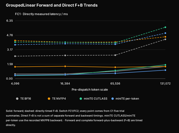
Figure 6. Qwen3-30B-A3B GroupedLinear on B300, warm static weights, five runs. Solid lines show forward, dashed lines directly measured F+B. Both miniTE paths use quantized backward in this figure. The horizontal axis is pre-dispatch token scale; this balanced workload is distinct from full-model routing.
miniTE per-token forward is approximately 1.09–1.43× faster than BF16, while its F+B in the figure is slower. BF16 backward makes miniTE per-token F+B approximately 1.2–1.3× faster than its own MXFP8-backward path. This directly motivates measuring complete operator cost before selecting backward precision.
Module Cost Across Workloads and Backward Precisions
Interactive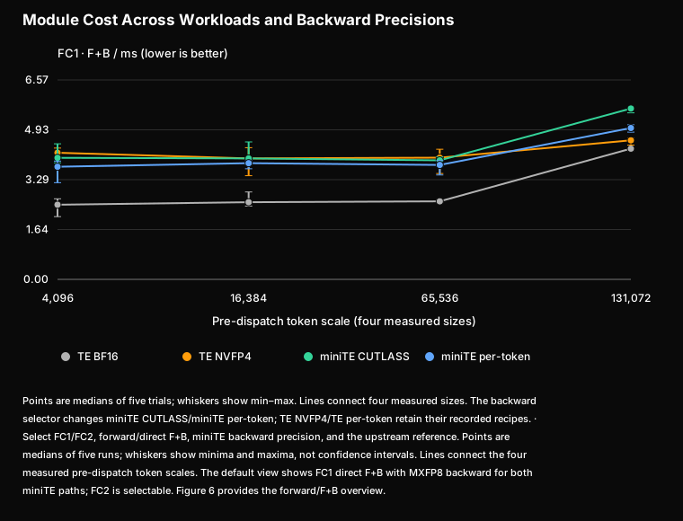
D11 · FC1/FC2 at Four Sizes: Complete Forward and Direct F+B Latencies
Forward
| Module | Configuration | Measurement | 4k ms | 16k ms | 64k ms | 128k ms |
|---|---|---|---|---|---|---|
| FC1 | TE BF16 | Forward | 0.504 | 0.515 | 0.801 | 1.329 |
| FC1 | TE NVFP4 | Forward | 1.295 | 1.349 | 1.250 | 1.327 |
| FC1 | miniTE CUTLASS | Forward | 0.336 | 0.396 | 0.895 | 1.508 |
| FC1 | miniTE per-token | Forward | 0.372 | 0.424 | 0.582 | 0.932 |
| FC2 | TE BF16 | Forward | 0.542 | 0.508 | 0.546 | 0.820 |
| FC2 | TE NVFP4 | Forward | 1.428 | 1.190 | 1.281 | 1.244 |
| FC2 | miniTE CUTLASS | Forward | 0.339 | 0.355 | 0.677 | 1.111 |
| FC2 | miniTE per-token | Forward | 0.389 | 0.415 | 0.565 | 0.753 |
Direct F+B with MXFP8 Backward
| Module | Configuration | Measurement | 4k ms | 16k ms | 64k ms | 128k ms |
|---|---|---|---|---|---|---|
| FC1 | TE BF16 | fwb | 2.461 | 2.543 | 2.572 | 4.309 |
| FC1 | TE NVFP4 | fwb | 4.174 | 3.986 | 4.011 | 4.583 |
| FC1 | miniTE CUTLASS | fwb | 4.006 | 3.987 | 3.923 | 5.631 |
| FC1 | miniTE per-token | fwb | 3.712 | 3.830 | 3.771 | 4.989 |
| FC2 | TE BF16 | fwb | 2.959 | 2.994 | 2.933 | 4.592 |
| FC2 | TE NVFP4 | fwb | 4.604 | 4.790 | 4.802 | 5.414 |
| FC2 | miniTE CUTLASS | fwb | 4.147 | 3.916 | 3.881 | 5.417 |
| FC2 | miniTE per-token | fwb | 3.875 | 3.915 | 3.907 | 5.056 |
Direct F+B with BF16 Backward
| Module | Configuration | Measurement | 4k ms | 16k ms | 64k ms | 128k ms |
|---|---|---|---|---|---|---|
| FC1 | miniTE CUTLASS | fwb | 2.975 | 2.966 | 3.253 | 5.473 |
| FC1 | miniTE per-token | fwb | 2.964 | 2.992 | 3.018 | 4.869 |
| FC2 | miniTE CUTLASS | fwb | 2.908 | 2.913 | 2.958 | 4.936 |
| FC2 | miniTE per-token | fwb | 3.158 | 2.943 | 3.088 | 4.636 |
Table 6-13. Five-run medians from the miniTE machine-readable records, shown to three decimal places. Backward configurations are kept separate. TE BF16/TE NVFP4 remain in their original configuration table because this BF16-backward supplement has no corresponding rows for them.
| Configuration | TE BF16 | TE NVFP4 | miniTE CUTLASS | miniTE per-token |
|---|---|---|---|---|
| 128k FC1 peak reserved GiB | 7.39 | 6.91 | 8.65 | 8.76 |
These memory values were measured in module tests under their stated timing and weight-cache settings. Learner peak memory is measured separately.
Raw data: main module records, BF16-backward records.
D12 · miniTE per-token Module Speedups over TE NVFP4
| Module | Mode | 4k | 16k | 64k | 128k |
|---|---|---|---|---|---|
| FC1 | Forward | 3.48x | 3.18x | 2.15x | 1.42x |
| FC1 | F+B | 1.12x | 1.04x | 1.06x | 0.92x |
| FC2 | Forward | 3.67x | 2.87x | 2.27x | 1.65x |
| FC2 | F+B | 1.19x | 1.22x | 1.23x | 1.07x |
Table 6-14. miniTE per-token/TE NVFP4 speedups for the corresponding configurations; >1 means miniTE per-token is faster. F+B uses each recorded backward path. miniTE per-token does not lead in every comparison at 128k FC1.
With the forward recipe fixed, miniTE per-token achieves a 2.46× geometric-mean expert-forward speedup over upstream TE per-token and 1.10× for direct F+B. The difference points to forward invocation and preparation as the main sources of implementation gains. Inputs are pre-permuted, FC2 activations are prepared outside the timer, and dispatch is excluded.
D13 · miniTE per-token/TE per-token by Workload Size and the amax Ablation
| Module | Mode | Workload size | TE per-token | miniTE per-token | miniTE per-token speedup |
|---|---|---|---|---|---|
| FC1 | Forward | 4k / 16k / 64k / 128k | 1.128 / 1.094 / 1.275 / 1.479 | 0.372 / 0.424 / 0.582 / 0.932 | 3.03x / 2.58x / 2.19x / 1.59x |
| FC1 | F+B | 4k / 16k / 64k / 128k | 3.873 / 3.916 / 3.846 / 5.066 | 3.712 / 3.830 / 3.771 / 4.989 | 1.04x / 1.02x / 1.02x / 1.02x |
| FC2 | Forward | 4k / 16k / 64k / 128k | 1.193 / 1.043 / 1.555 / 1.747 | 0.389 / 0.415 / 0.565 / 0.753 | 3.06x / 2.52x / 2.75x / 2.32x |
| FC2 | F+B | 4k / 16k / 64k / 128k | 4.603 / 4.507 / 4.488 / 6.234 | 3.875 / 3.915 / 3.907 / 5.056 | 1.19x / 1.15x / 1.15x / 1.23x |
Table 6-15. Module latencies and speedups from five runs. Numerical-equivalence checks hold the forward recipe fixed; the corresponding records specify environment and backward paths.
The amax skip-K1 simulation is neutral or slightly slower at most sizes, spanning approximately 0.81–1.11×. It excludes producer gains and retains preparation overhead, so it cannot independently establish the effect of full producer–consumer fusion. The dense layout is measured together with other optimizations; its individual contribution remains unmeasured.
| module | mode | Workload size | miniTE per-token amax off | miniTE per-token amax on | on vs off |
|---|---|---|---|---|---|
| fc1 | Forward | 4k | 0.372 | 0.459 | 0.81x |
| fc1 | Forward | 16k | 0.4241 | 0.4586 | 0.925x |
| fc1 | Forward | 64k | 0.5823 | 0.6166 | 0.944x |
| fc1 | Forward | 128k | 0.9319 | 0.8365 | 1.114x |
| fc1 | fwb | 4k | 3.7122 | 3.8659 | 0.96x |
| fc1 | fwb | 16k | 3.8303 | 3.8542 | 0.994x |
| fc1 | fwb | 64k | 3.7713 | 3.8175 | 0.988x |
| fc1 | fwb | 128k | 4.9888 | 4.9196 | 1.014x |
| fc2 | Forward | 4k | 0.3894 | 0.4017 | 0.969x |
| fc2 | Forward | 16k | 0.4145 | 0.4407 | 0.941x |
| fc2 | Forward | 64k | 0.5655 | 0.5927 | 0.954x |
| fc2 | Forward | 128k | 0.7534 | 0.7842 | 0.961x |
| fc2 | fwb | 4k | 3.8746 | 3.9556 | 0.98x |
| fc2 | fwb | 16k | 3.9151 | 3.995 | 0.98x |
| fc2 | fwb | 64k | 3.9069 | 3.8958 | 1.003x |
| fc2 | fwb | 128k | 5.0562 | 5.1263 | 0.986x |
Table 6-15b. miniTE per-token module-level skip-K1 simulation. Statistics follow the module test; producer gains are excluded.
Data and runs: module ablation records.
D14 · Upstream TE per-token Full-Model Timing and Configuration Scope
| Configuration | tokens/s(3 trials) | paired speedup vs TE per-token | Max reserved (MB) |
|---|---|---|---|
| TE per-token | 23125 / 23150 / 22346 | — | 122572 |
| TE BF16 | 25545 / 24531 / 23385 | 1.06x | 119914 |
| TE NVFP4 | 25863 / 23653 / 23291 | 1.04x | 122672 |
| miniTE per-token (mxfp8-bwd) | 27493 (run 0 reference) | 1.19x (run 0 paired) | 138458 |
| miniTE per-token (bf16-bwd) | 33464 / 31417 / 34429 | 1.45x | 133398 |
Table 6-16. Three-run full-model comparison. Approximately 1.45× is the timing ratio between these configurations, not an implementation-only gain at the same recipe.
TE per-token quantizes non-expert layers as well and uses its native per-token NVFP4 backward path. miniTE per-token is expert-only and is tested with MXFP8/BF16 backward. The TE per-token runs also record gradient norms around 1e8–1e11, leaving very small actual updates after clipping. Timing and learning behavior are both retained; the speed ratio does not describe equivalent learning paths.
See the TE per-token full-model records.
Profiling explains the transition from local to full-model performance: host metadata preparation, gaps between grouped calls, expert communication, and non-GEMM operations all affect update time. Contiguous layouts reduce organization overhead, while model tests include real routing and surrounding costs.
D15 · Representative Profiles: Multi-Tensor Calls and Grouped GEMM
How dispatch and routing affect downstream GEMM scheduling. In the supplementary record's first microbatch of Step 8, routing from real weights and inputs is more uniform, while mock routing from random weights and inputs is concentrated. Both use 4,096 input tokens per rank, top-k=8, and 131,072 routed tokens within the EP group. We first compare expert distributions at this common token budget:
| Load metric | Real | Mock | Interpretation |
|---|---|---|---|
| Experts with tokens | 126/128 | 24/128 | Mock concentrates tokens on fewer experts |
| Zero-token experts | 2 | 104 | The number of participating experts differs |
| CV of GroupedLinear M | 0.19 | 0.66 | The recorded Real GEMM row counts are more uniform |
M is the token-row count of an expert GEMM. CV is the standard deviation divided by the mean under the same statistical definition; we retain the recorded GroupedLinear M statistic instead of reconstructing it from global expert counts. More participating experts create more matrix-multiplication problems to prepare and schedule. Host API and kernel profiles help explain that cost:
| Call metric | Real | Mock | Interpretation |
|---|---|---|---|
| cuBLASLt heuristic calls / cumulative time | 148,000 / 6.26 s | 32,000 / 1.02 s | Real has approximately 4.6× as many calls |
| Median time per heuristic call | 2.9 µs | 2.9 µs | Similar medians, different call counts |
| nvte_multi_tensor_gemm calls / median time | 4,608 / 2.29 ms | 4,590 / 0.44 ms | Similar counts; Real's median is approximately 5.2× |
| nvjet kernel calls | 114,000 | 4,600 | Real has approximately 25× as many calls |
The first table identifies this microbatch's routing load; the second preserves call counts, cumulative times, and per-call medians from the accompanying profile. Cumulative times are not treated as this one microbatch's wall time or added directly to GPU kernel times.
The same token budget is split into more GEMM problems. For matching expert matrix shapes, the main GEMM arithmetic scales with the sum of expert token-row counts. Real and Mock have the same token total, but Real distributes it across 126 active experts and Mock across 24. Real therefore has a smaller average M per expert and more nonempty problem entries. Its lower CV indicates a more balanced distribution, while preparation and scheduling also depend on problem count and granularity. Many smaller GEMMs have less computation over which to amortize fixed preparation and launch costs.
cuBLASLt algorithm selection repeatedly runs on the host. The original profile identifies AlgoGetHeuristic as a major BF16 bottleneck. The multi-stream, multi-tensor path still performs repeated algorithm selection and prepares shapes, layouts, and call parameters for expert problems. Both heuristic medians are 2.9 µs, but Real has approximately 4.6× as many calls, indicating that repeated work drives the extra cost. Outer nvte_multi_tensor_gemm counts are similar, while the expert problems and preparation inside each call differ. Real's median call time is consequently 2.29 ms, approximately 5.2× Mock's.
More fine-grained kernels lengthen the submission chain. Real has approximately 25× as many nvjet kernels as Mock, showing different GPU call organization for the same token budget. If CPU algorithm selection, argument preparation, and launch submission become the bottleneck, additional streams may not hide the GPU's wait for its next tasks. This is the CPU bubble to examine in that path. The counts directly support increased preparation and scheduling work; the duration of GPU gaps still requires the corresponding timeline.
Dense grouped GEMM targets this preparation and scheduling chain. Section 5's contiguous buffers, device-side offsets and metadata, and reusable allocations put expert problems on one grouped scheduling path, reducing host-side slicing, list assembly, argument construction, and repeated organization. These changes affect the work surrounding GEMM and the complete call time, so the observed difference should be interpreted together with the implementation path. Actual speed ratios remain based on comparable module or learner timings, with real weights and routing used for both BF16 and low-precision evaluation.

Recorded profile
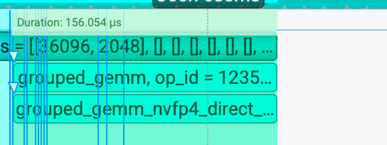
Recorded profile
Figure 7. Representative profiles illustrating invocation structure. The screenshots do not supply paired timings with matching shapes and timers, so 3.594 ms and 156µs are not divided to report a speedup. Performance comes from the module/learner measurements above.
6.5 Rollout and Online RL: System Gains and Remaining Costs
The sampler is first tested at fixed output workload. Eight engines use real DAPO prompts, generate exactly 1024 tokens with EOS ignored, and independently select concurrency 64 after a sweep for each configuration:
| Configuration | Aggregate output tokens/s | Mean TPOT | Throughput ratio |
|---|---|---|---|
| BF16 | 49,119.1 | 10.21 ms | 1.000× |
| NVFP4 | 80,675.8 | 6.05 ms | 1.642× |
Table 6-17. Fixed-output serving. BF16 uses Triton MoE; NVFP4 uses FlashInfer TRT-LLM/ModelOpt FP4 and per-token scaling. This measures the sampling stack rather than isolating miniTE training operators.
Sampling Capacity at a Fixed Workload
Interactive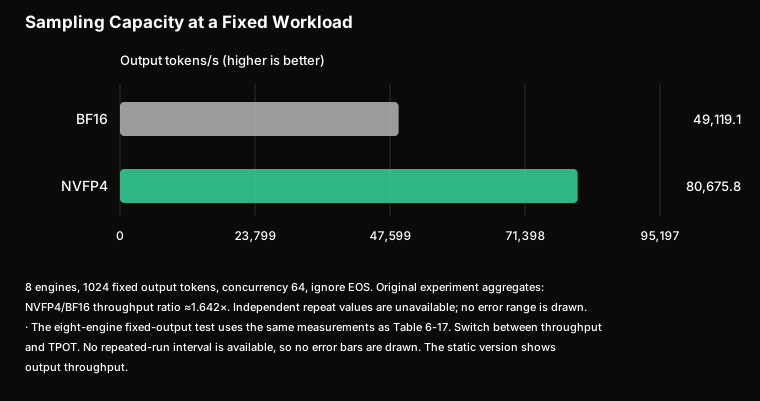
D16 · Eight-Engine Request Rates, Per-Engine Throughput, and Serving Protocol
| variant | BEST concurrency | final sum out tok/s | Mean output / engine | sum req/s | mean TPOT | vs peer |
|---|---|---|---|---|---|---|
| NVFP4 | 64 | 80675.8 | 10084.5 | 78.78 | 6.05 ms | 1.64× vs BF16 |
| BF16 | 64 | 49119.1 | 6139.9 | 47.97 | 10.21 ms | baseline |
Table 6-18. Complete serving results. At fixed output length, request rate and output-token throughput describe the same workload.
The static memory fraction is 0.6 and piecewise CUDA graphs are disabled. Requests use a chat template, unpadded inputs, no rate limit, cache flushing, and context limit 8192. A single-engine sweep uses 64 prompts and concurrency 1–96; the selected concurrency 64 is then tested with 512 prompts across eight engines. Single-engine peak throughput is approximately 10206.8 tokens/s for NVFP4 and 6063.5 for BF16, separate from the eight-engine aggregate main result.
Complete RL also connects learner updates and weight synchronization to generation. For a sequential workflow without overlap,
When stages overlap, measured wall time is the reference. Table 6-19 reports the recorded stages for BF16, native TE NVFP4, and miniTE per-token:
| Configuration | Steady-state steps | Train s | Conversion/sync s | Two-stage total s |
|---|---|---|---|---|
| BF16 | 11 | 47.04 | 9.94 | 56.98 |
| TE NVFP4 | 10 | 44.70 | 50.88 | 95.58 |
| miniTE per-token, BF16 backward | 10 | 42.56 | 55.26 | 97.82 |
Table 6-19. Mean online RL stage times. Train includes log-probability recomputation and actor training. The two-stage sum is not a full iteration. TE NVFP4 uses its native backward configuration; miniTE per-token explicitly disables backward quantization.
Compute Gains and Conversion/Synchronization Cost
Interactive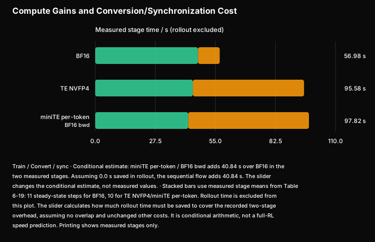
miniTE per-token Train is approximately 1.11× faster than BF16 and TE NVFP4 approximately 1.05×. Conversion/synchronization is approximately 5.56× and 5.12× slower, respectively. miniTE per-token adds 40.84 seconds across these two stages. In this run, rollout gains did not offset synchronization cost, making conversion and transfer important targets for further optimization.
This negative result is useful: faster low-precision operators do not ensure lower system integration costs. Independent serving ratios cannot replace rollout time measured over the same run window, and summing these two stages does not yield a complete RL speedup.
D17 · Three RL Configurations, Measurement Windows, and Relative Speeds
All configurations use colocated deployment on one 8×B300 node, with one GPU per sampler engine. Performance IDs 0–1 are discarded. BF16 averages steps 2–12 (11 steps); miniTE per-token/TE NVFP4 each average steps 2–11 (10 steps). Values are arithmetic means.
| Configuration | Train speedup over BF16 | Sync time / BF16 sync time | Forward / sampling | Backward |
|---|---|---|---|---|
| BF16 | 1.000× | 1.000× | BF16, Triton MoE | BF16 |
| TE NVFP4 | 1.052× | 5.119× | Native TE expert NVFP4; ModelOpt/FlashInfer sampler | Native recipe, DBQ unset |
| miniTE per-token | 1.105× | 5.559× | miniTE expert per-token; same NVFP4 sampler | DBQ=1, BF16 |
Table 6-20. Ratios have explicit directions. The earlier 0.90× value is the miniTE per-token/BF16 Train-time ratio; speed is its reciprocal, not a full-RL result. TE NVFP4 and miniTE per-token use the same type of NVFP4 rollout configuration; the serving table is not independently remeasured for each.
Key result · §6.5In the eight-engine fixed-output test, miniTE per-token serving throughput is about 1.64× BF16.
6.6 What the Experiments Establish
Together, these experiments explain miniTE's implementation choices. Operator and gradient checks support interfaces, layouts, and backward precision. Module forward and direct F+B timings locate local costs. Real-text learner tests establish whether these choices reduce complete update cost. Serving and online RL tests reveal the additional constraints of weight conversion and synchronization.
Low-bit training benefits must therefore be validated at multiple levels: numerical correctness, sustained learning, faster local computation, and manageable integration cost. We retain core measurements and complete configuration comparisons at each level, using miniTE test records for performance results.
7. Using and Extending miniTE
7.1 Integrating Existing Models through Linear Interfaces
The implementation package is miniTransformer, and the linear layer is miniTE's basic integration unit. Linear, LayerNormLinear, and GroupedLinear provide ordinary projections, combined normalization and linear computation, and MoE expert computation. Existing Megatron wrappers can connect to these modules, or users can pass parameters constructed from a named recipe directly:
import torch
from miniTransformer.module.config import get_qlinear_params
from miniTransformer.module.linear import Linear

params = get_qlinear_params("nvfp4_per_token")
layer = Linear(
    1024, 1024,
    bias=False,
    params_dtype=torch.bfloat16,
    device="cuda",
    qlinear_params=params,
)
Recipe selection determines the numerical path; module integration determines which model layers use miniTE. The MoE launcher sets both for its miniTransformer backends. GroupedLinear imposes output-dimension and grouped-layout constraints and does not support sequence parallelism. Integration should check the specific model and parallel configuration.
miniTE retains TE/Megatron checkpoint parameter naming and compatibility interfaces. The current extra-state interface does not restore all TE internal quantization state. Parameter-loading compatibility and full internal-state compatibility are validated separately.
7.2 Explicit Recipes and Precision Boundaries
Version 1.0.0 uses names describing numerical behavior. Users select a training recipe with MINITE_RECIPE or construct independent parameters and operators with get_qlinear_params:
| Named recipe | Forward and scaling | Backward and use |
|---|---|---|
nvfp4_per_token | Per-token NVFP4; TE weight scaling | MXFP8 backward; first-use example |
nvfp4_per_token_bf16_bwd | Per-token NVFP4 | Dedicated TE-style BF16 backward operator |
nvfp4_cursor2_cutlass_v2 | Per-token activations, per-expert tensor weight amax; CUTLASS V2 | MXFP8 backward; custom grouped path |
nvfp4_block | NVFP4 block scaling | NVFP4 backward; block-scaling recipe |
nvfp4_per_token_w_per_tensor | Per-token activations, per-expert tensor weight amax | Weight-scaling ablation |
unquantized | Dtype controlled by layer parameters | Quantization disabled for high-precision comparison |
Table 9. Selected named entries in version 1.0.0. Performance experiments retain their own source revisions, forward/backward precision, and quantization coverage; names select the current software configuration.
For an integrated training program:
MINITE_RECIPE=nvfp4_per_token python train.py
Here train.py denotes the user's training entry point. Expressing the report's miniTE per-token BF16 layer-bypass choice through the current named interface gives:
MINITE_RECIPE=nvfp4_per_token DISABLE_BACKWARD_QUANT=1 python train.py
This layer bypass and the dedicated nvfp4_per_token_bf16_bwd operator are implemented and recorded separately. Speeds of both miniTE paths in Section 6 belong to the original experimental paths. The dedicated operator requires its own performance measurements. Historical reproduction also uses the original revision's launch configuration and fixes sampler quantization, checkpoint conversion, expert-only coverage, and TE revision.
7.3 Diagnostics as Part of Extension Development
Configuration checks begin before constructing a model. Run these commands from the miniTransformer repository root:
python -m miniTransformer recipes
python -m miniTransformer describe nvfp4_per_token
python -m miniTransformer doctor --recipe nvfp4_per_token
bash develop/script/moe_training_e2e.sh \
  --backend mini_nvfp4_per_token --profile off --dry-run
recipes and describe expose names, dependencies, and backward overrides without Torch or TE. doctor inspects visible CUDA GPUs, TE quantizer arguments, selected dense/list grouped interfaces, and operator imports. --dry-run prints the recipe, relevant environment, and complete command without starting training or creating log/cache directories. Actual runs record the recipe name, forward/backward settings, layout request, and configuration source in run_meta.json.
All 21 CPU compatibility checks for this interface update passed, covering resolution, conflicting selectors, inspection without GPU dependencies, backend aliases, dry-run, and metadata. Added GPU equivalence tests cover independent configurations, forward/backward behavior on supported Dense/GroupedLinear paths, and the two BF16 backward choices. They have not been run locally in this update. Numerical and performance results in Section 6 retain their original experiment identities.
When extending a low-precision path, we check operators, then modules and cross-framework behavior, and finally complete training. Tensor hooks collect activation, weight, output, and gradient statistics. Profiling locates kernel costs, call gaps, and allocation. Dump/compare scripts examine MoE intermediates and token log probabilities. A new recipe declares its purpose and dependencies in the registry, connects its operator through the existing parameter factory, and follows these numerical and runtime checks.
The repository README covers setup, layer integration, and launch examples; the bilingual recipe guides document selection and override rules. Model conversion, sampling, and evaluation require their own pinned versions and settings. Current software interfaces and historical experiment configurations are recorded separately.
8. Discussion: From Numerical Alignment to End-to-End Learning
The experiments address low-precision RL through two approaches: TRIAGE changes updates in the presence of mismatch, while miniTE reduces execution differences and compute cost. Neither resolves every issue. The next questions are whether faster computation yields end-to-end savings, and whether closer numerical agreement produces better learning.
8.1 Weight Updates and Synchronization Remain a Bottleneck
Here, update weight means converting, transferring, and loading the trained weights into the sampler. This remains a major bottleneck in the configurations we measured. Faster learner updates and rollouts do not imply a proportional reduction in complete RL iteration time. In the run reported in Section 6.5, conversion and synchronization costs offset the gains from faster sampling.
Further optimization should consider parameter representations, quantization and packing, transfer, loading, and synchronization frequency together. Possible directions include reusing low-precision representations within the same weight version, combining conversion with transfer, and overlapping synchronization with sampling under explicit version control. Less frequent synchronization can save transfer time but increases policy staleness. These choices should be evaluated using complete iteration time and task performance under matched training budgets. Online amax and deeper operator fusion also need evaluation within this end-to-end scope.
8.2 Why Does Low Precision Remain Sensitive After Operator Alignment?
Matching operators and quantization recipes removes some execution differences. Matching their names alone, however, does not guarantee identical floating-point computation across input shapes, batches, and parallel configurations. Floating-point addition is not associative: changes in reduction order, fusion boundaries, or tiling can change the result. A fixed execution path can be deterministic. The remaining question is where perturbations arise when execution conditions change and how they affect subsequent updates.
Our alignment experiment and long-run evaluations expose two sides of this problem. The strict alignment configuration reduces gap to approximately 10⁻⁸, while miniTE’s long-run learning and checkpoint evaluations do not match BF16 in every comparison. These results use different configurations and measurement scopes, but together they show why numerical agreement and final learning quality must be evaluated separately. Why can seemingly small perturbations be more damaging in the low-precision configurations we tested?
Candidate mechanisms include persistent error bias, rounding transitions near coarse quantization boundaries, MoE routing changes, and the accumulated response of gradient clipping and optimizer state. These remain hypotheses. More informative experiments would hold the model and data fixed, control the location, direction, and correlation of perturbations, and compare subsequent updates and long-run reward in BF16 and low precision, rather than relying on a single-step average gap.
8.3 Optimize Updates and Final Learning Outcomes
Mean log-probability difference cannot be converted linearly into reward. Similar average gaps can occur on different tokens, advantage signs, and response segments, with different effects on updates. A small gap also does not guarantee useful exploration or gradient signal. TRIAGE’s directional analysis offers one starting point. Further work can directly examine how errors alter updates, testing corrections through reward and evaluation scores under matched data, update, and wall-clock budgets.
The community’s approaches are broadening too. Together AI’s Score Centering (SC) adds a correction that removes mismatch-induced drift from the policy gradient and can be combined with importance sampling [17]. The Qwen team’s TRACE uses rollout-side quantization outcomes to guide training-side FP4 rounding and compresses the guidance information [18]. SC changes the gradient estimator; TRACE coordinates quantization decisions. TRACE still targets alignment, but both works expand the available interventions beyond matching operator implementations.
For miniTE, this means supporting joint experiments on update rules, precision allocation, and sampling policy alongside controlled, comparable numerical execution. We hope the community will investigate how to preserve task-relevant learning signal, suppress bias that compounds across updates, and translate these changes into end-to-end gains. The goal is better learning within a given resource budget, not simply a smaller consistency metric.
Appendix A. Experimental Setup and Statistics
A.1 Supplementary Algorithm and Training Materials
TRIAGE's method and results follow the release manuscript and its diagnostic appendix. Checkpoints are those in Table 3, with equal weight across five mathematics benchmarks. Updated 4B means are 58.26% for BF16 and 58.49% for TRIAGE; TRIAGE scores 53.03% at the shared step-300 checkpoint.
Characterization uses separate diagnostic runs: updates 1–324 for 4B and 1–724 for 30B, with maximum completion lengths 16,384 and 20,480. The 4B analysis uses direct learner–sampler gaps; 30B uses residual gaps after routing replay. Fixed tail thresholds over valid tokens in the healthy stage are −0.24208 and −0.03949, respectively.
These diagnostic runs use DAPO-Math-17K, learner seed 1234, rollout/data seed 42, 16 prompts per iteration, 16 responses per prompt, and GBS 256. They use RHT and gradient stochastic rounding; these numerical settings differ from miniTE's practical path, where the options are disabled. Detailed windows, length sensitivity, one-step update audits, and randomization controls are in the diagnostic appendix.
TRIAGE materials are used for algorithmic outcomes. Its image was not tuned to the same level as the miniTE performance environment, so its throughput is not used as a miniTE upper bound or an algorithm-overhead baseline.
A.2 Supplementary Long-Run RL and Checkpoint Evaluation
Figure 5 and Table 6-8 use the following training configuration and evaluation protocol:
| Item | Setting |
|---|---|
| Model and data | Qwen3-30B-A3B-Base; DAPO-Math-17K, math reward |
| Objective | GRPO; token-wise TIS in non-strict configurations |
| Seeds | Training seed 1234; rollout shuffle seed 42 |
| Batch | 32 prompts per iteration, 16 responses each; GBS 512 |
| Generation | Temperature 1.0, top-p 1.0, top-k disabled, maximum response 20,480 |
| Parallelism and allocation | 8 nodes, 8 actor GPUs each; TP/PP/CP/EP/ETP = 1/1/1/4/1; colocated actor/sampler |
| Optimizer | Adam, learning rate , no warmup; weight decay 0.1, , gradient clipping 1.0 |
| Memory policy | Full activation recomputation, dynamic microbatches; distributed precision-aware optimizer, CPU offload and overlapping transfer |
| TIS and clipping | Token-wise TIS clipped to [0,2]; policy update ratio [0.80,1.28]; routing replay disabled |
| Evaluation | Step 999; temperature 0.7, top-p 1.0, maximum generation length 20,480 |
| Repetitions and metrics | Six evaluations per AIME; four each for MATH-500, GSM8K, IFEval; IFEval Prompt-level Strict |
Table A1. Supplementary miniTE long-run protocol. This differs from the fixed-text learner test on one 8×B300 node. Repeated checkpoint evaluations do not increase the number of training seeds.
The three main configurations cover steps 0–999, with one trajectory each and centered 21-step means. Figure 4 retains the four-panel plot with 15-step smoothing; the accompanying paper also contains a two-panel presentation of a related alignment experiment with 21-step smoothing. Each caption retains its own convention. Strict alignment changes several execution components together and removes TIS; its timing is separate from learner performance tests.
A.3 Fixed-Text miniTE Learner Tests
| Item | Setting |
|---|---|
| Model and hardware | Qwen3-30B-A3B, one 8×B300 node |
| Parallelism and shape | TP/PP/CP/EP = 1/1/1/4; sequence 4096; micro-batch 1; GBS 128 |
| Workload | 524,288 tokens per update; 16 accumulated microbatches |
| Data and initialization | 657 frozen 4097-token DAPO sequences; same BF16 checkpoint; seed 20260913 |
| Software | PyTorch 2.11.0+cu130, CUDA 13.0.88, NCCL 2.28.9, Megatron-Core 0.16.0rc0 |
| Megatron | Revision 52153937, integration patches for the experiment |
| Core revision | miniTE 953f17f9; ten independent processes, no permutation fusion |
| Optimized revision | miniTE b641179; dense, GEMM-kind, permutation fusion and amax reuse |
| TE | Early eaca54e9, later 8ea5a92d handles zero-token experts; nonempty-group paths checked |
| TE per-token | 690ffea4 with CUDA 13 build fixes, separate environment |
Table A2. Fixed-text performance protocol. Data construction includes approximately 4.3-fold repetition. Activation recomputation, offload, and CUDA graphs are disabled. Expert-padding costs of quantized paths are included in timing.
The core protocol runs 20 updates per process, uses five warmup updates, and measures updates 6–15. Each run's throughput is 524,288 divided by median update time. Across ten runs, the maximum and minimum are removed before averaging. Speedups are first paired by run ID and then trimmed in the same way.
The optimized protocol uses one process per configuration and 17 updates. After two warmups, the maximum and minimum of the remaining 15 update times are removed. Throughput is 524,288 tokens divided by the mean of the retained times; speedups use the same-round baseline. The estimators are reported separately. Core run 3 experienced interference from an idle serving process, and affected minimum observations are removed under the predefined trimming rule. All ten records and revision differences remain in the miniTE summary.
Table 6-9 uses paired speedups from ten independent runs. The 1.334× value is the trimmed mean of per-run ratios; 1.344× is the ratio of aggregate throughput means. The later fusion experiment uses a different revision and configuration and is reported separately.
A.4 Module, Serving, and RL Stage Timing
Module tests use one GPU, 32 local experts, four pre-dispatch token sizes, and five independent process runs with warm static weights. Dispatch is excluded and FC2 activations are prepared beforehand. Module-forward gains are distinct from learner speedups. Upstream TE per-token has different full-model quantization coverage and backward precision from miniTE; its full-model comparison is not used to isolate implementation gains.
Serving uses fixed output length 1024, ignore_eos=true, context limit 8,192 tokens, static memory fraction 0.6, and disabled piecewise CUDA graphs. A single engine uses 64 prompts to sweep concurrency 1, 2, 4, 8, 16, 32, 48, 64, and 96. Both configurations select 64 before processing 512 prompts across eight engines.
Colocated RL tests use one 8×B300 node and one GPU per engine. BF16 statistics cover performance steps 2–12; miniTE covers 2–11. Learner timing includes log-probability computation and actor training. Weight updates include Megatron→SGLang synchronization and miniTE's BF16→NVFP4 conversion. The two-stage sum excludes full rollout and other orchestration work.
API and fused-layout checks compare encodings, scales, and outputs at fixed shapes and configurations. Bitwise agreement at these boundaries does not establish full-model batch invariance. Earlier swizzle failures and the production miniTE per-token checks use different shape constraints and are interpreted separately.
Appendix B. TRIAGE Method Conventions
We use response-level normalization from the release manuscript: compute a weighted token-loss mean within each response, then average across responses. With valid-token mask and detached gate weight ,
The fixed gate uses 64-token segments. For negative-advantage segments, the mean-tier weight is 0.1 when mean gap is below −1.5, 0.3 for [−1.5, −0.5), and 1.0 otherwise. If valid tokens in the segment satisfy , the tail weight is . The smaller of the two segment weights is applied only to negative-gap tokens. Other tokens retain weight 1.
Repair uses 128-token segments within positive-advantage responses and applies a one-sided pseudo-Huber penalty beyond the negative boundary. Masks, segment normalization, and derivatives are described in the TRIAGE method appendix and main method section.
Component ablations branch from the full-TRIAGE step-300 checkpoint and compare continued training. The complete figure is in the TRIAGE ablation. These are continuation comparisons rather than ablations trained from scratch.
The diagrams and interactive presentation draw on The 4-bitter Lesson and the LMSYS Blackwell low-precision RL article [15,16]. Constructed examples and conditional calculations are identified separately.
References
[1] NVIDIA. Pretraining Large Language Models with NVFP4. 2025; updated 2026. arXiv:2509.25149.
[2] Cursor Research. Composer 2 Technical Report. 2026. arXiv:2603.24477.
[3] Guangming Sheng et al. HybridFlow: A Flexible and Efficient RLHF Framework. EuroSys 2025. arXiv:2409.19256.
[4] Zhihong Shao et al. DeepSeekMath: Pushing the Limits of Mathematical Reasoning in Open Language Models. 2024. arXiv:2402.03300.
[5] An Yang et al. Qwen3 Technical Report. 2025. arXiv:2505.09388.
[6] Qiying Yu et al. DAPO: An Open-Source LLM Reinforcement Learning System at Scale. 2025. arXiv:2503.14476; DAPO-Math-17K dataset.
[7] Lianmin Zheng et al. SGLang: Efficient Execution of Structured Language Model Programs. NeurIPS 2024. arXiv:2312.07104.
[8] Mohammad Shoeybi et al. Megatron-LM: Training Multi-Billion Parameter Language Models Using Model Parallelism. 2019. arXiv:1909.08053.
[9] NVIDIA Transformer Engine. Add NVFP4 per-token quantization recipe, PR #3045. 2026. Implementation and discussion.
[10] Zhaopeng Qiu et al. FP8-RL: A Practical and Stable Low-Precision Stack for LLM Reinforcement Learning. 2026. arXiv:2601.18150.
[11] Karl Cobbe et al. Training Verifiers to Solve Math Word Problems. 2021. arXiv:2110.14168; official GSM8K repository.
[12] Dan Hendrycks et al. Measuring Mathematical Problem Solving With the MATH Dataset. 2021. arXiv:2103.03874. For the MATH-500 split, see Hunter Lightman et al., Let's Verify Step by Step, 2023, arXiv:2305.20050, and the official split description.
[13] Mathematical Association of America. Official AMC page and AIME introduction. Results use the AIME 2024, AIME 2025, and AMC23 evaluation versions recorded in the experiments.
[14] Jeffrey Zhou et al. Instruction-Following Evaluation for Large Language Models. 2023. arXiv:2311.07911.
[15] Ziang Li et al. The 4-bitter Lesson. humans&, 2026-07-10. Article and interactive examples.
[16] Ziang Li, humans& and Miles Team. Towards Blackwell-Native 8-bit and 4-bit RL: End-to-End MXFP8 and NVFP4 RL in Miles. LMSYS, 2026-07-29. Article and format explanation.
[17] Martin Marek and Max Ryabinin. Score Centering Stabilizes Off-policy Reinforcement Learning. 2026. Paper.
[18] Xin Wang et al. TRACE: Rollout-Guided Quantization-Aware Training for FP4 Reinforcement Learning of MoE Language Models. 2026. Paper.