Model Merging Scaling Laws in Large Language Models
ABSTRACT
This work studies empirical scaling laws for language model merging measured by cross-entropy. Across 10,866 merged models, base sizes from 0.5B to 72B, nine domains, and four methods, the paper identifies a compact floor-plus-tail power law that links model size and expert count. The law explains why most merging gains arrive early, why variability shrinks as more experts are included, and how to plan expert count under a budget.
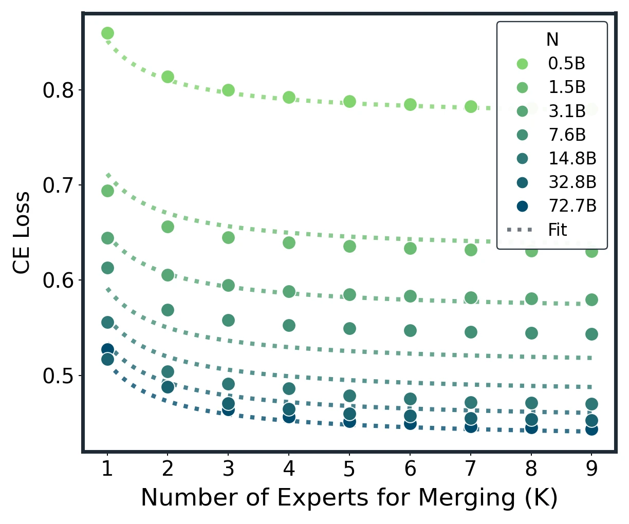
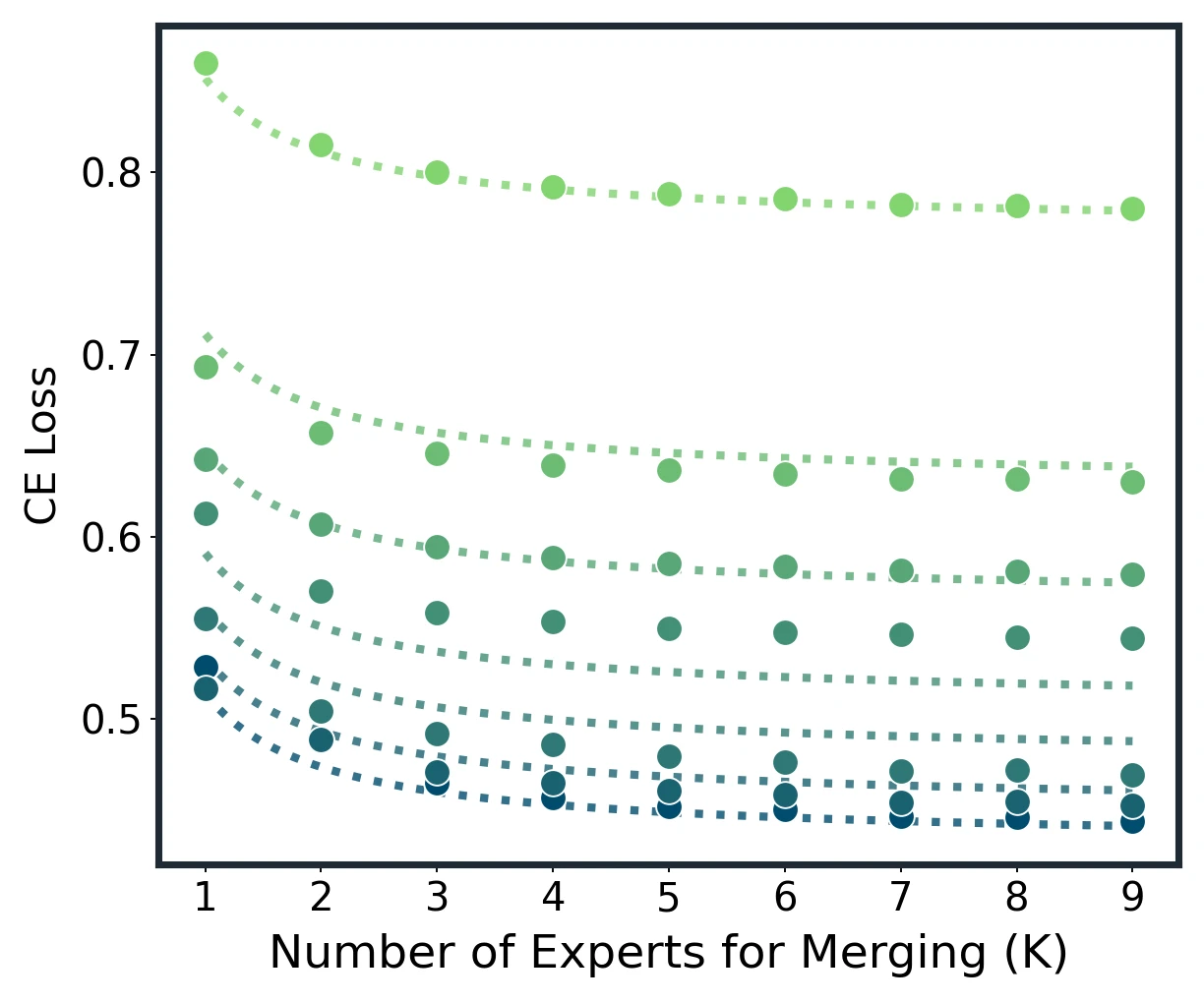
Model merging scaling law across Average, Task Arithmetic, TIES, and DARE. Dots are measured results; dotted lines are unified-law fits.
Abstract
This work studies empirical scaling laws for language model merging, measured by cross-entropy. Although model merging is widely used in practice, it lacks a quantitative rule that predicts returns as more experts are added or as the base model scales.
The paper identifies a compact power law that links model size and expert count. The size-dependent floor decreases with model capacity, while the merging tail exhibits clear diminishing returns in the number of experts. The law holds in-domain and cross-domain, fits measured curves across diverse architectures and methods, and explains two robust regularities: most gains arrive early, and variability shrinks as more experts are included.
The resulting law enables predictive planning: estimating how many experts are needed to reach a target loss, deciding when to stop adding experts, and trading off scaling the base model versus adding experts under a fixed budget.
Introduction
Large language models are often specialized by fine-tuning on different domains, producing multiple domain experts. Model merging combines these experts in weight space to synthesize a single model without retraining. It supports modular pipelines, can approximate joint training at a fraction of the cost, and enables composition under privacy or compute constraints.
However, merging is still largely empirical. Practitioners experiment with expert subsets, orders, and normalization rules, often at substantial computational expense. Unlike pretraining, where scaling laws guide tradeoffs among model size, data, and compute, merging has lacked a quantitative account that predicts convergence as experts are added.
This paper introduces a predictive merging scaling law that couples base model size with the number of merged experts :
Larger base models lower the size-dependent floor and shrink the tail amplitude. Adding experts yields steep early improvements, then tapers roughly as .
Contributions
- Unified scaling law: a compact floor-plus-tail law links base size and expert count, and applies consistently in in-domain and cross-domain settings.
- Large-scale validation: the law is validated over 10,866 merged models, seven Qwen2.5 sizes from 0.5B to 72B, nine domains, and four merging methods.
- Theory: a leading-order inverse- tail and variance contraction are derived under equal-normalized composition of effective updates.
- Operational recipe: a lightweight three-point fitting procedure predicts the full merge curve and recommends an efficient expert count for budget-aware planning.
Background and Setup
Model Merging
Model merging integrates independently trained models into a single model by aggregating parameters. The paper studies:
- Average: direct equal-weight averaging of task vectors;
- Task Arithmetic (TA): scaled task-vector composition;
- TIES: trimming, electing, and disjoint merging to reduce interference;
- DARE: random masking and rescaling of task vectors.
The unified view is:
Here, is the base model, is the task vector for expert , is a selected subset of experts, and is the method-specific preprocessing map.
Expert Models and Data
The controlled experiments start from Qwen2.5 base models at 0.5B, 1.5B, 3B, 7B, 14B, 32B, and 72B. The authors train nine domain specialists using data from Mixture-of-Thoughts and OpenScience:
- mathematics: algebra, analysis, discrete mathematics and combinatorics, geometry and topology, number theory;
- science: biology, physics, chemistry;
- code.
Evaluation uses token-level cross-entropy. For each domain, 30M held-out tokens are scored and averaged. For each , the expected merge loss is computed over all possible -expert subsets when feasible, or over a large uniform sample for larger models.
Scaling Law Results
Expected Loss Construction
For a fixed base size and expert count , there are possible expert subsets. Each subset can yield a distinct merged model. The expected merge loss is:
Individual subset losses vary, but the per- mean forms a smooth curve with diminishing returns.
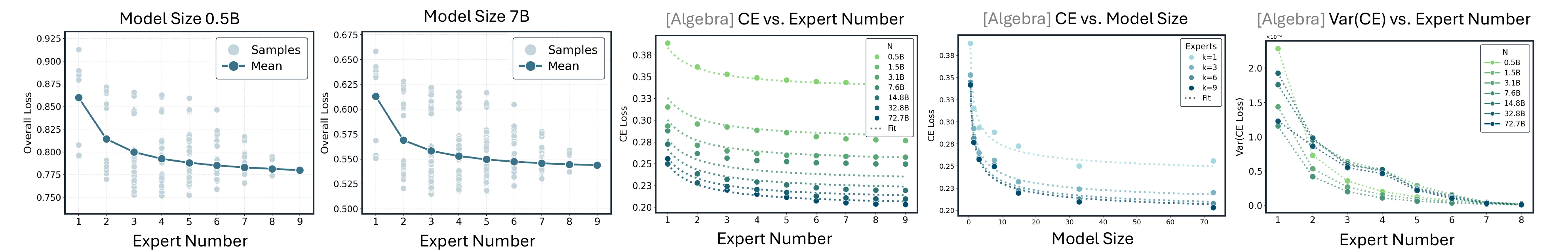
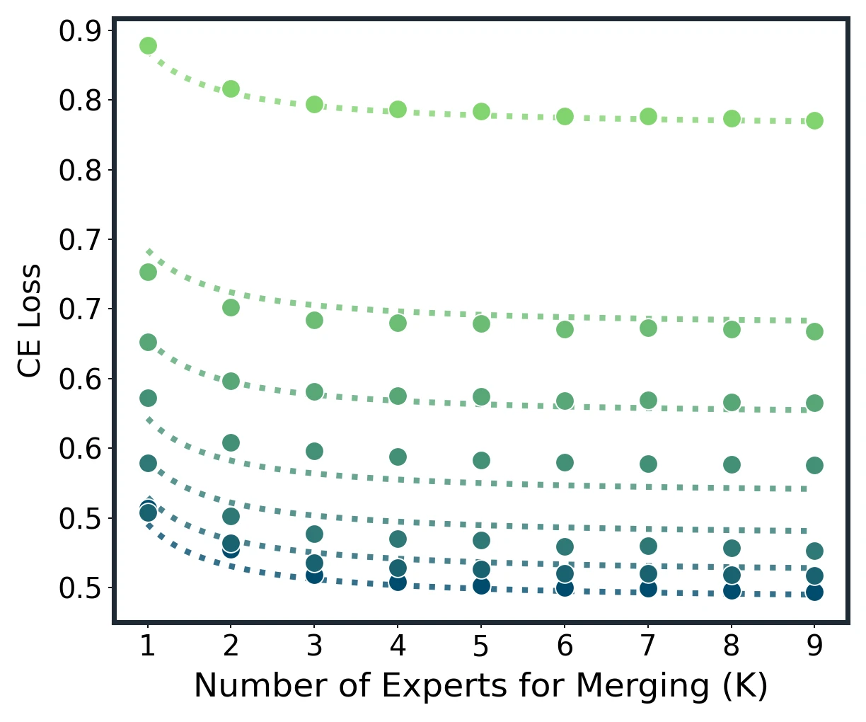
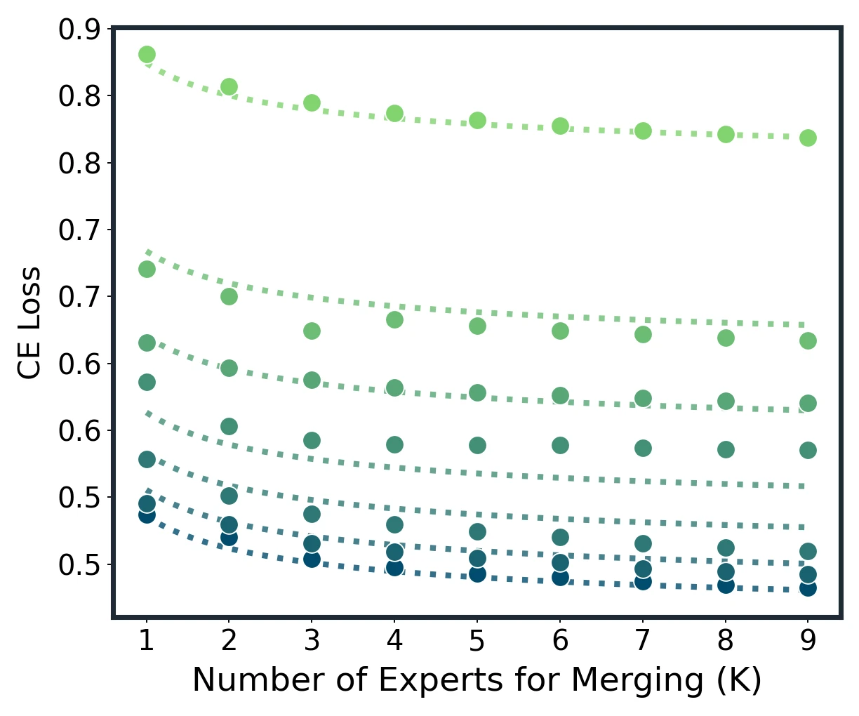
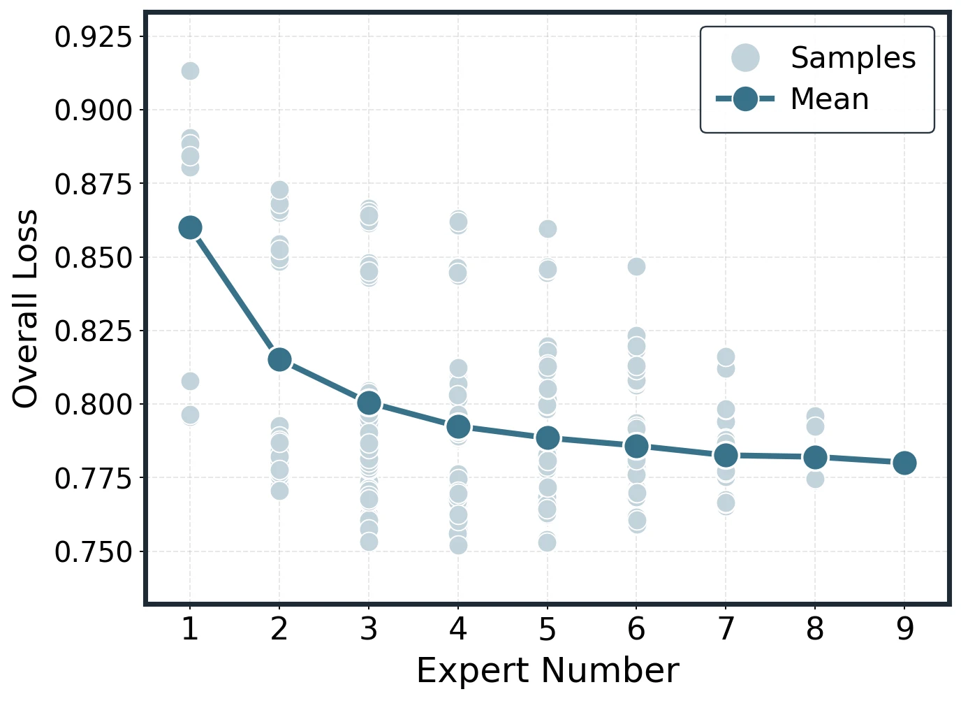
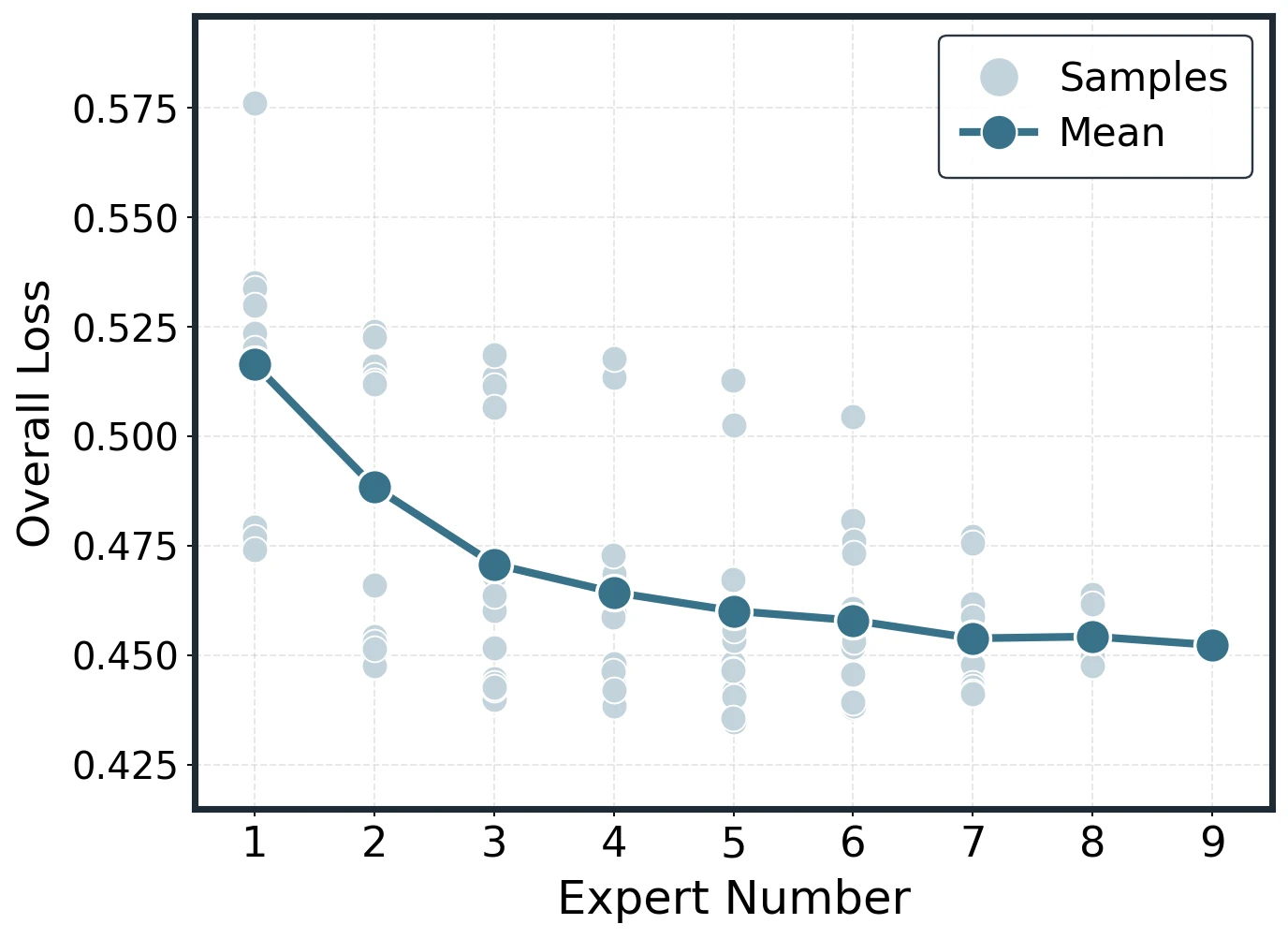
Empirical construction of expected loss and in-domain scaling on Qwen2.5 models.
Unified Empirical Law
The expected loss follows:
The model-size dependencies are:
This gives a simple interpretation:
- bigger models lower the asymptotic floor;
- bigger models shrink the remaining tail;
- adding experts gives early gains that rapidly diminish.
Across methods and settings, the paper reports near-unity fits, with over fitted points.
Merging Versus Multitask SFT
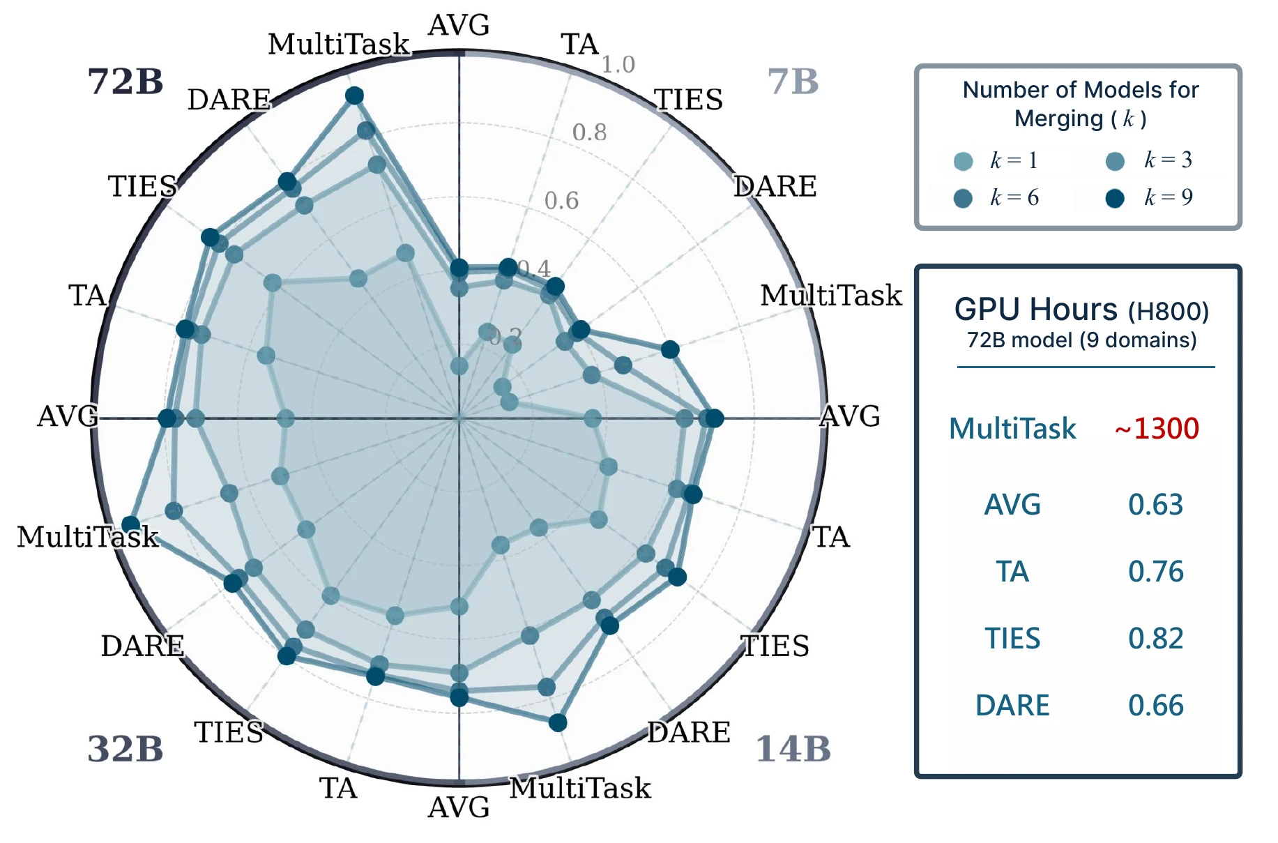
Merging approaches multitask SFT performance while using negligible GPU-hours.
The paper directly compares merging with multitask SFT under normalized loss and GPU-hours. On a 72B model with nine domains, multitask SFT costs roughly 1300 H800 GPU hours, while merging costs less than one GPU-hour for the reported methods.
Theory
The paper explains the inverse- tail with an average-case argument. Under equal normalization, merging corresponds to averaging task update vectors. As increases, the variance of the averaged update shrinks as . A second-order Taylor expansion of the loss converts this variance reduction into expected-loss improvement of the same order.
For each fixed model size , the theorem states:
with:
and:
Here, and are the mean and covariance of task updates in the merged subspace. For TIES and DARE, the same analysis is applied to effective updates after method-specific preprocessing.
The variance result is:
This explains why merging more experts improves not only average performance but also reliability.
Core Findings
Larger Models Are Easier to Merge
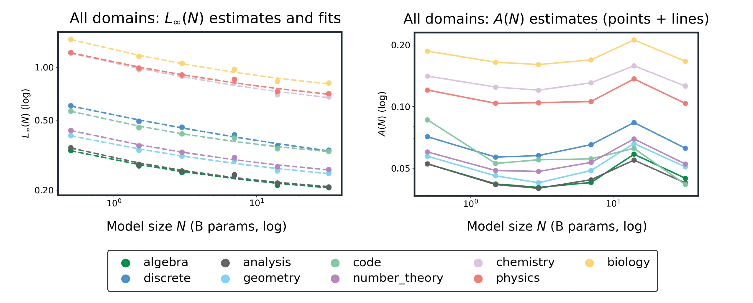
Per-domain floors and tail amplitudes as functions of model size.
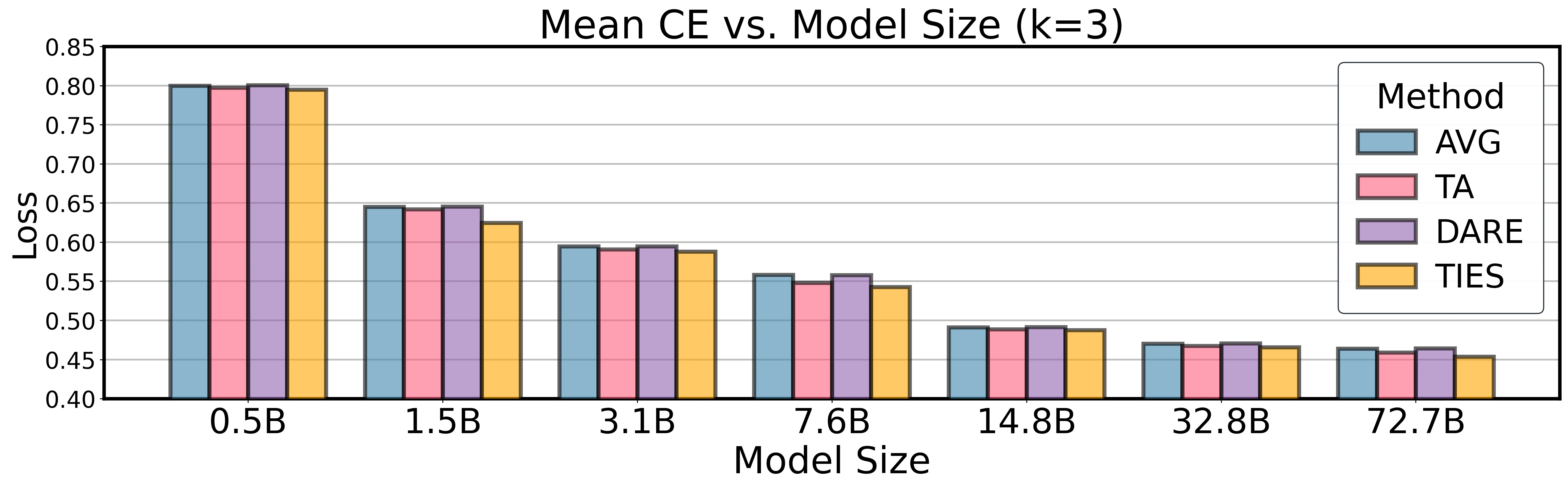
At fixed , larger models have lower CE and need fewer experts to approach the floor. At , domain-averaged CE drops from 0.739 at 0.5B to 0.430 at 32B, a 41.9% reduction.
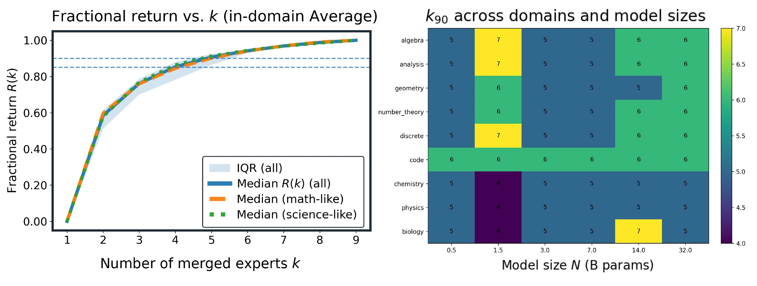
Most gains arrive early: k=5 and k=6 cross the 85% and 90% return thresholds.
The paper finds that and reach about 85% and 90% of the measured improvement. Roughly 60% of the nine-expert pool is enough to recover over 90% of the gains.
Mixing Domains Helps Generalization
Cross-domain merging follows the same law as in-domain merging. Gains are monotone in , steep early, and flatten into a tail. Diverse donor domains reduce domain-specific bias and help pooled generalization under the same scaling form.
Method Gaps Shrink at Scale
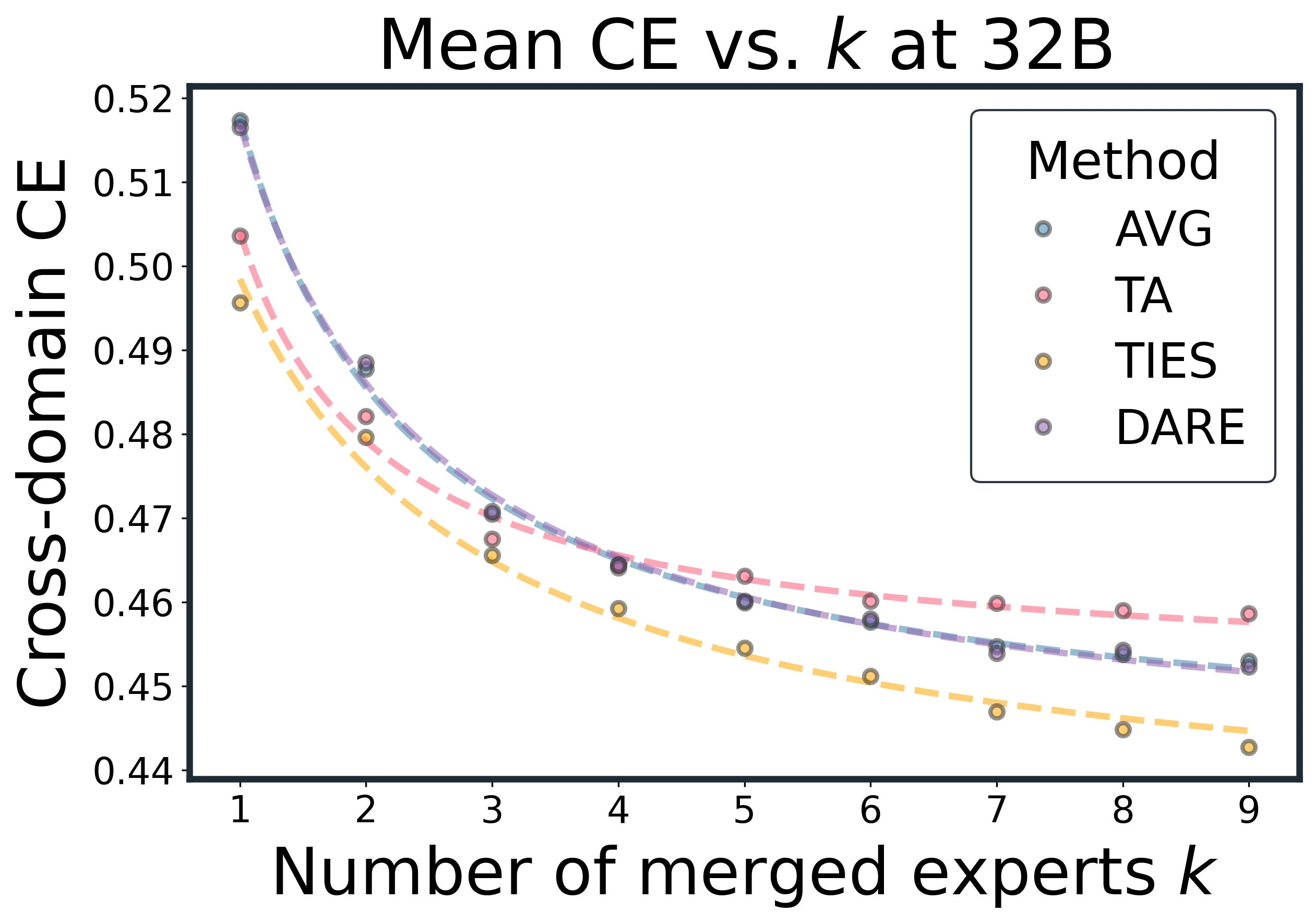
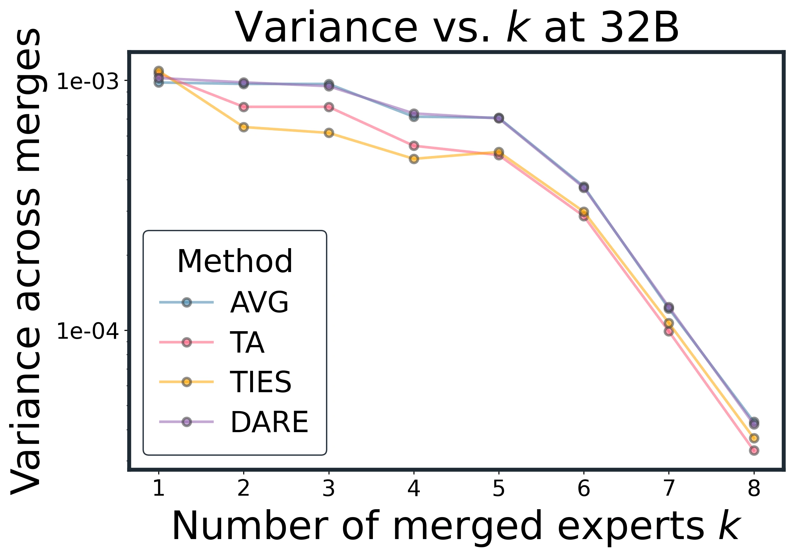
Method sensitivity diminishes at scale: small early-k gaps narrow quickly, while variance contracts for all methods.
At larger and , method gaps compress quickly. Early advantages for TA or TIES at small shrink to a tight band by , with differences below about 2%. Variance shows similar convergence.
Practical Recipe
Three Points Predict the Curve
The paper fits:
using only three early points: . This forecast closely tracks the full trajectory.
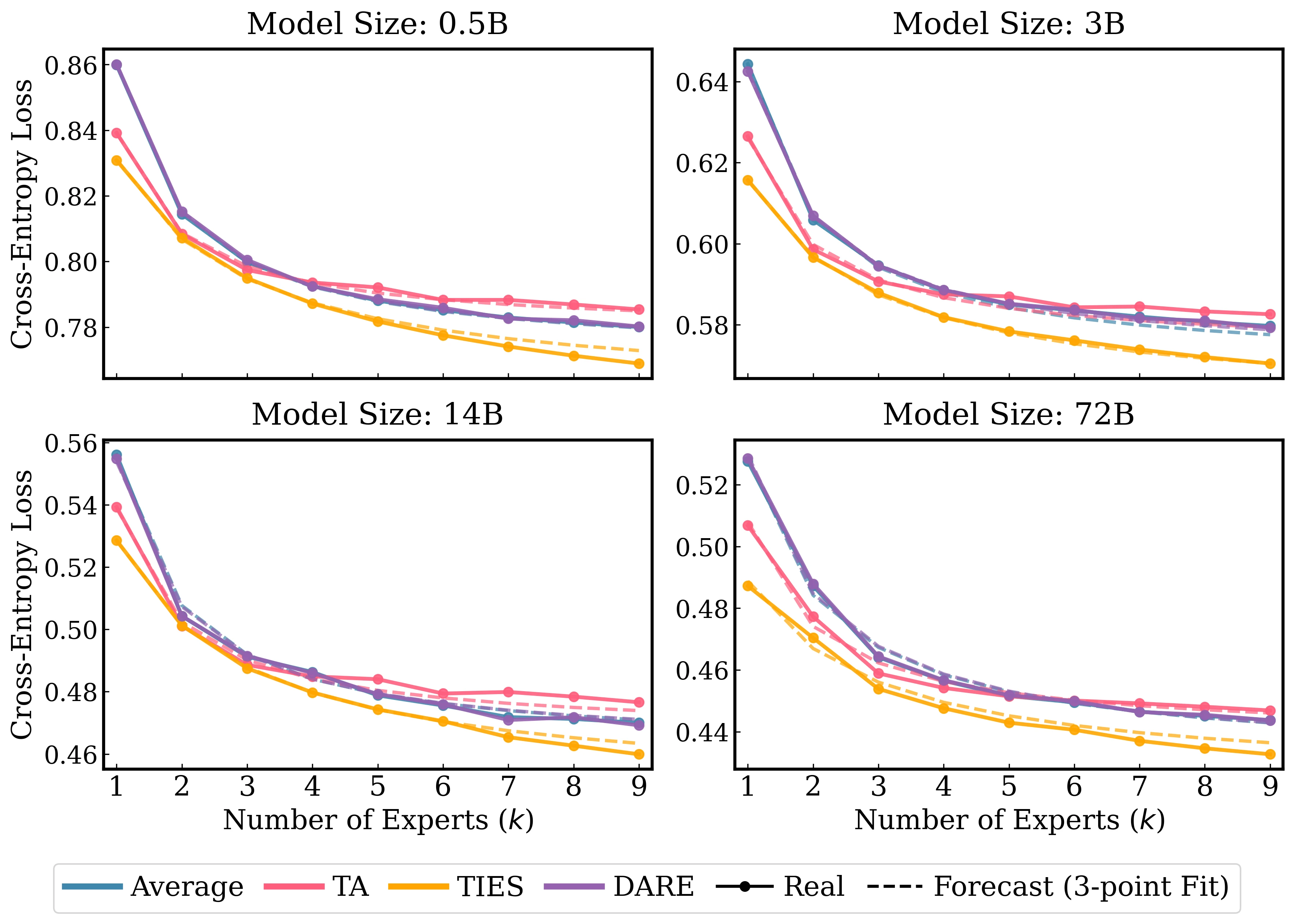
Fitting on k=1,2,4 closely predicts the full k-curve.
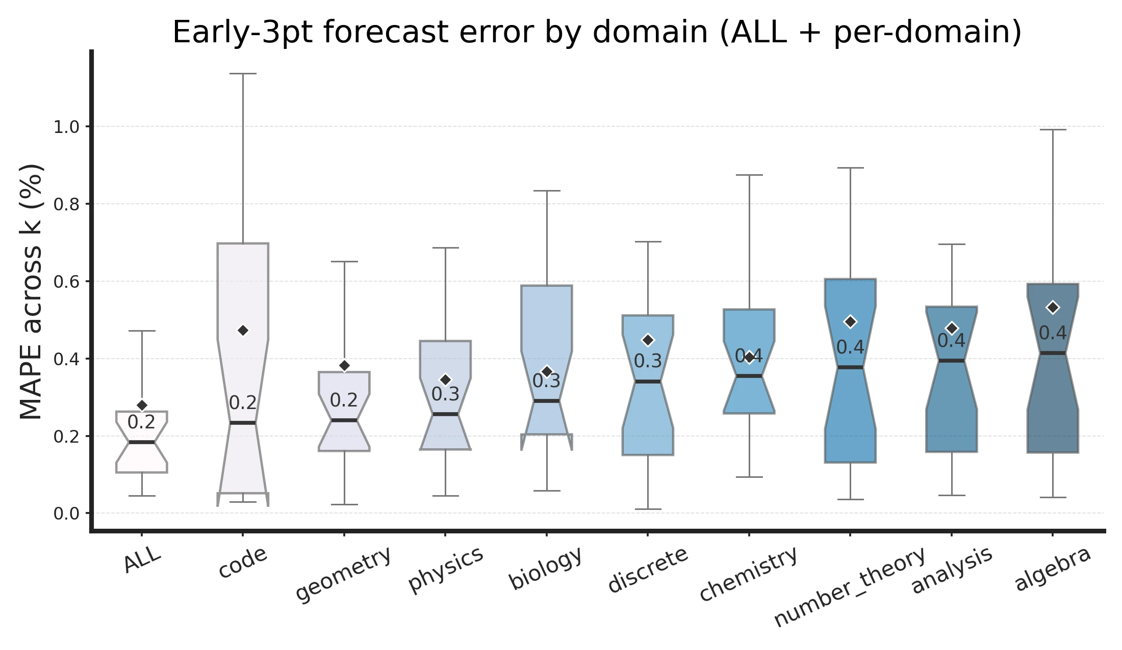
Forecast errors stay low and recommended k concentrates around small values.
This turns merge planning into a lightweight measurement problem: evaluate a few early expert counts, fit the curve, then decide when additional experts no longer justify their cost.
Merge Order Matters Less as k Grows
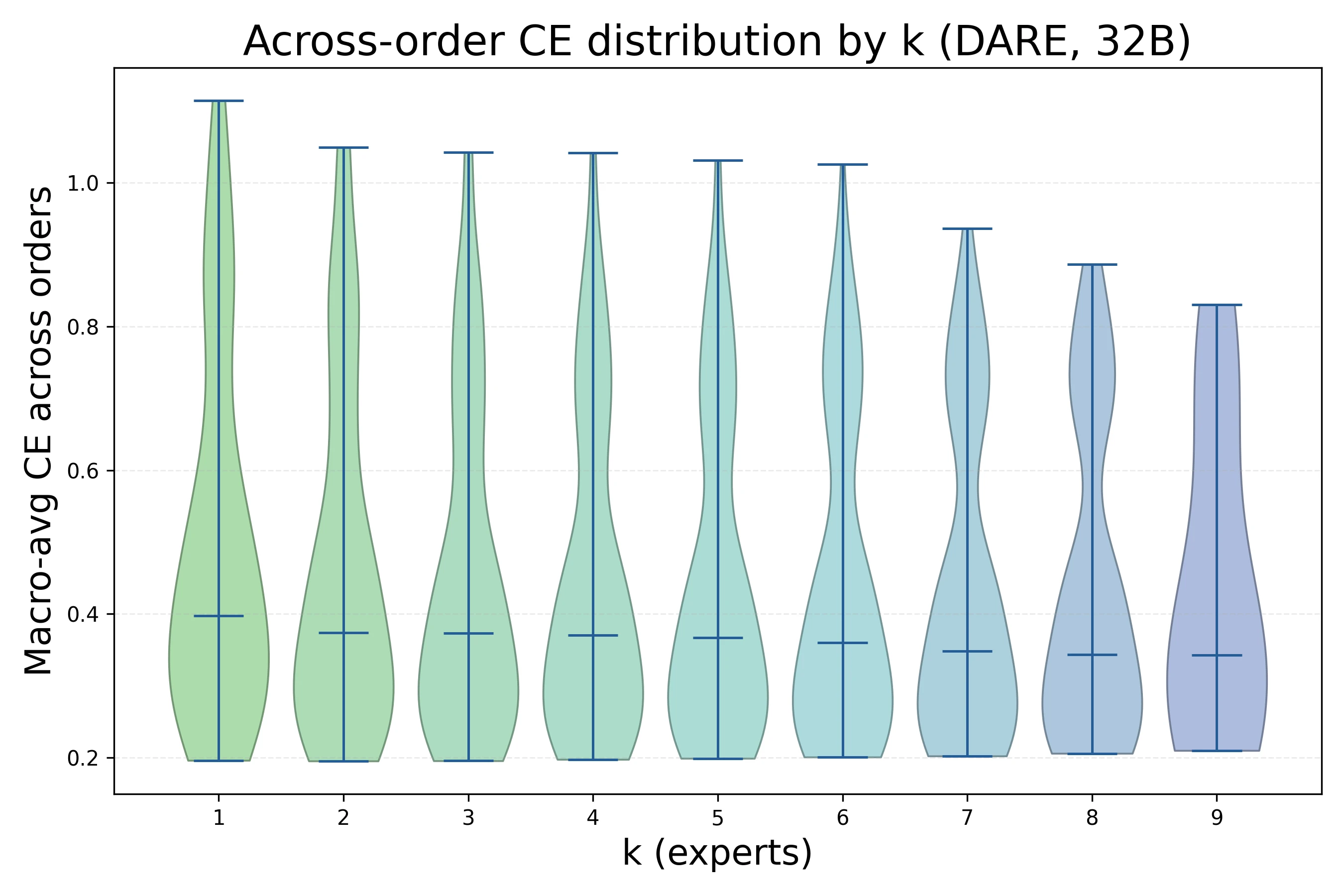
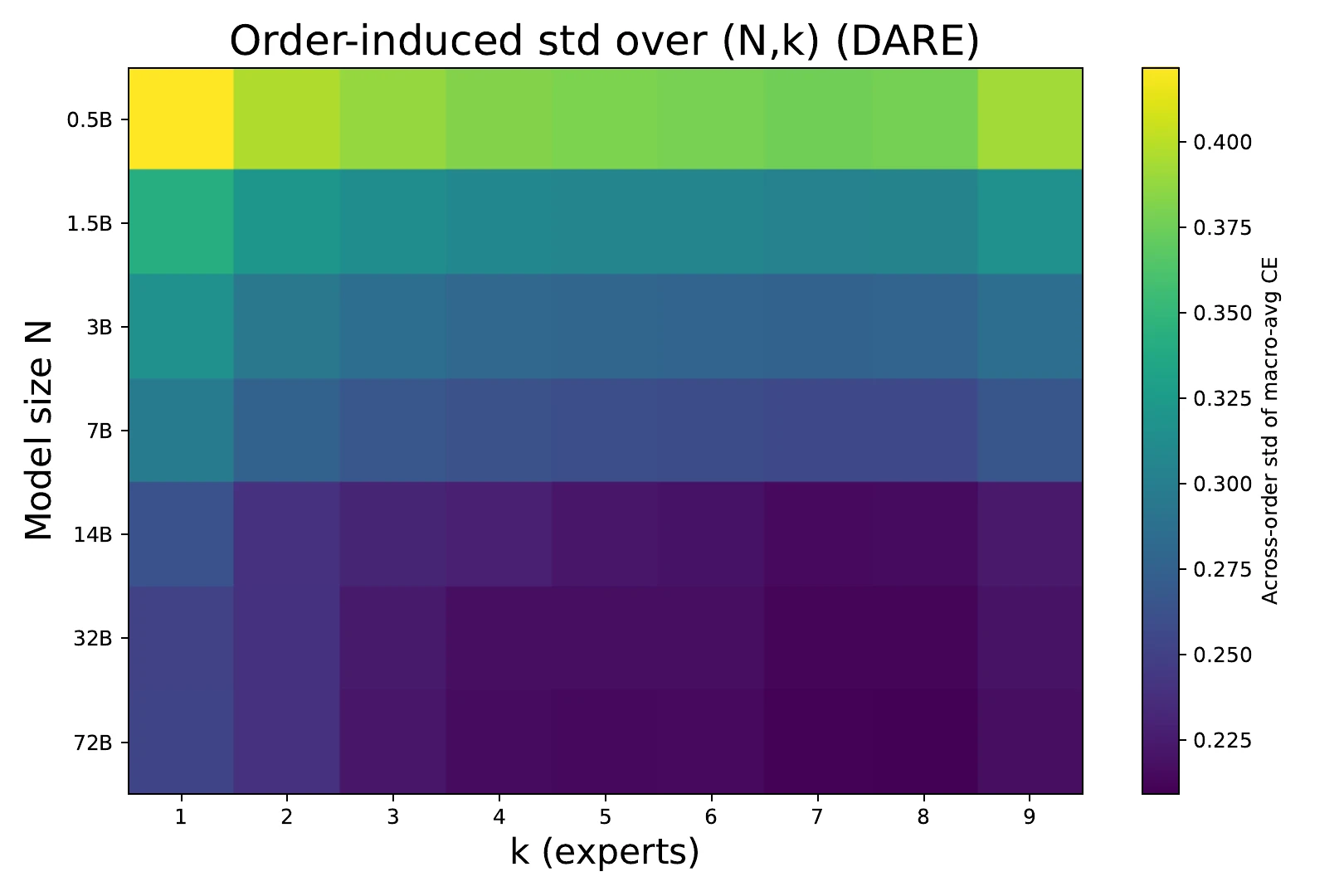
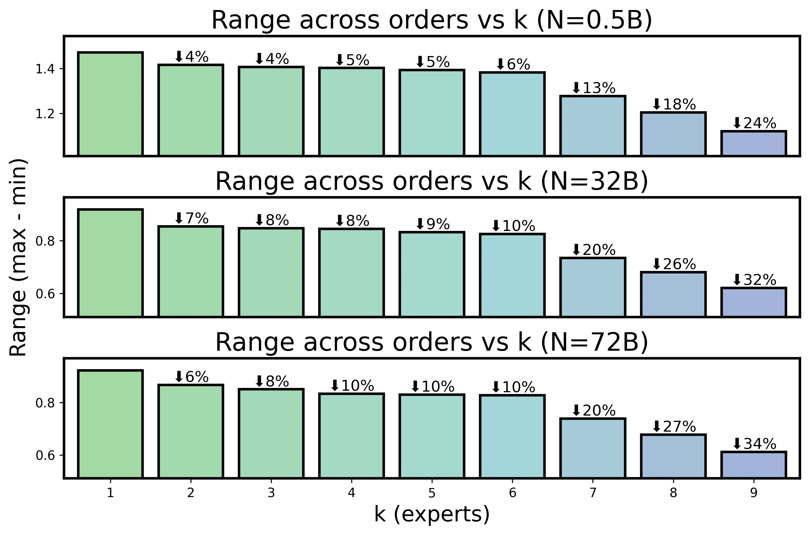
Order sensitivity contracts rapidly as k increases under DARE.
Under DARE, across-order dispersion shrinks rapidly with . Once , the spread from merge order is small compared with early method gaps and the scaling-law floor.
The Law Transfers Across Backbones
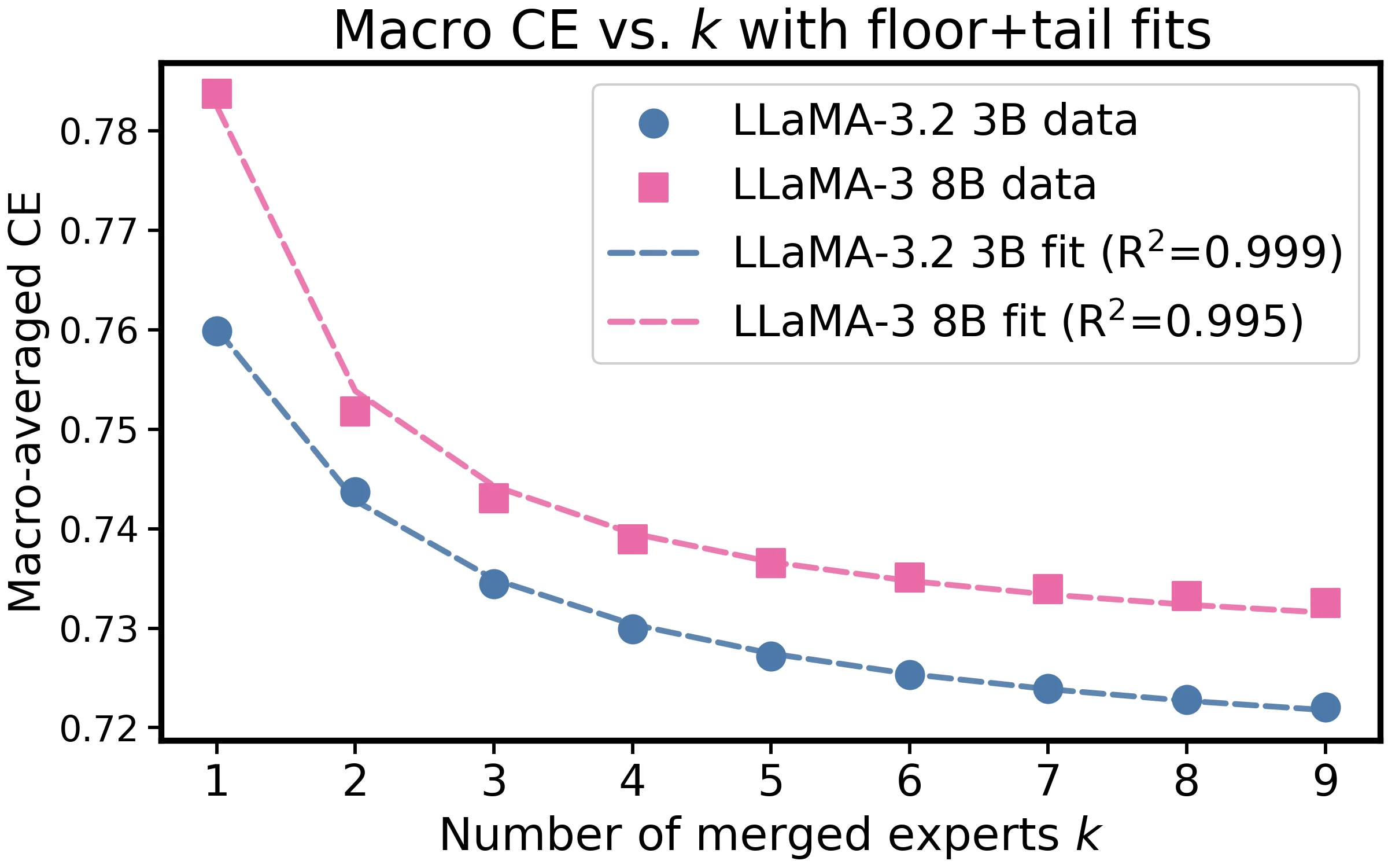
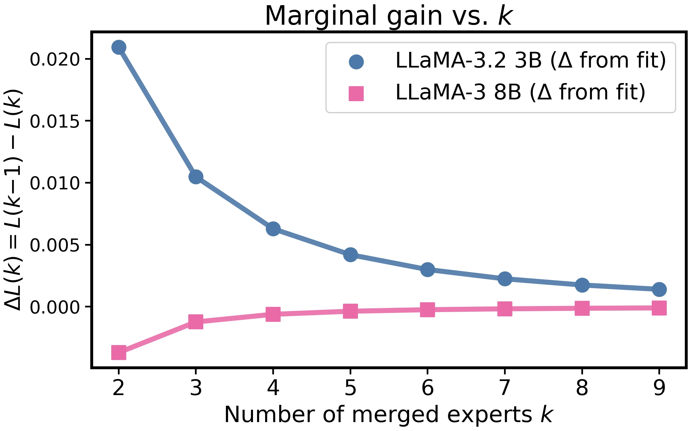
The same inverse-tail law holds on LLaMA-3.2 3B and LLaMA-3 8B.
On LLaMA-3.2 3B and LLaMA-3 8B, macro CE again follows the same inverse-tail law. The paper reports for LLaMA-3.2 3B and for LLaMA-3 8B.
Appendix: Reproducibility
All models and datasets used in the study are publicly available. The paper describes the data sources, methodological choices, and evaluation protocol in the main setup section, then gives extra implementation details and hyperparameters in the appendix. The complete source code is provided as supplementary material, and the checkpoints are planned for release.
Statement of LLM Usage
The authors report using an LLM only as an editing tool for syntax correction and stylistic polishing. The LLM was not used to generate or revise the central research ideas, design experiments, or organize the paper.
Model Merging Recipes
The paper represents all merging methods with:
| Method | Effective update | Extra parameters | ||
|---|---|---|---|---|
| Average | 1 | none | ||
| Task Arithmetic | 0.8 | none | ||
| TIES | trim, elect, disjoint merge | 1 | density | |
| DARE | 1 | drop rate |
This table is the implementation-level bridge between the empirical law and specific merging algorithms: Average and TA differ mainly by scale, TIES modifies the effective update by sparsifying and resolving signs, and DARE uses random masking plus rescaling before the normalized merge.
Detailed Theory
The appendix proves the inverse-tail law for a fixed model size . The proof assumes the loss is twice continuously differentiable near the base model, the Hessian is Lipschitz, task vectors have finite sixth moment, and equal-normalized weights satisfy .
Let:
The mean-corrected step has:
Taylor expanding at gives:
Substituting and taking expectation removes the linear term and leaves:
The main text writes the intercept and tail at the base point using a PSD curvature surrogate :
The appendix then bounds the base-point approximation error by the Hessian Lipschitz constant, , and curvature-surrogate mismatch. At the empirical granularity used in the paper, these are absorbed into fitted and , yielding:
For variance, the same expansion decomposes:
The leading linear term contributes:
The quadratic term contributes , the remainder contributes , and the covariance terms are lower order. Thus, in the non-degenerate case:
If the linear term degenerates, the proof gives a tighter variance bound, with tightness when the quadratic fluctuation is nonzero on the covariance subspace.
Expert Model Details
The expert models are trained with a shared recipe so that the scaling study isolates merging behavior rather than changing expert capacity. The hyperparameters are:
| Hyperparameter | Value |
|---|---|
| Batch size | 16 |
| Learning rate | |
| Warmup ratio | 0.05 |
| Epochs | 2 |
| Maximum sequence length | 16,384 |
| Optimizer | Adam with offloading |
| Precision | bfloat16 |
| Gradient checkpointing | enabled |
| ZeRO stage | 3 |
Evaluation uses token-level cross-entropy. For each domain, 30M validation tokens are sampled. The domain-specific loss is the average negative log-likelihood over validation tokens:
For every , there are possible expert selections, and each selection may produce a different merged model. The expected loss is therefore computed over all subsets when feasible, and by sampling when the model size makes exhaustive merging too expensive.
The authors explicitly distinguish this weight-space merging study from model-fusion methods such as InfiGFusion and InfiFPO, which require data and additional training.
Sampling Algorithm
For large models, the paper samples diverse merge permutations instead of enumerating every possible subset/order. The algorithm initializes with the canonical sequence , adds the reverse sequence when , then repeatedly samples 1000 random candidate permutations and chooses the one maximizing its minimum Hamming distance to the already selected set.
Input: k, base sequence s = [1, 2, ..., 9]
P <- {s}
if k >= 2:
  P <- P union {reverse(s)}
for i = 3 ... k:
  C <- 1000 random shuffles of s
  pi* <- argmax_pi min_{pi' in P} HammingDistance(pi, pi')
  P <- P union {pi*}
return P
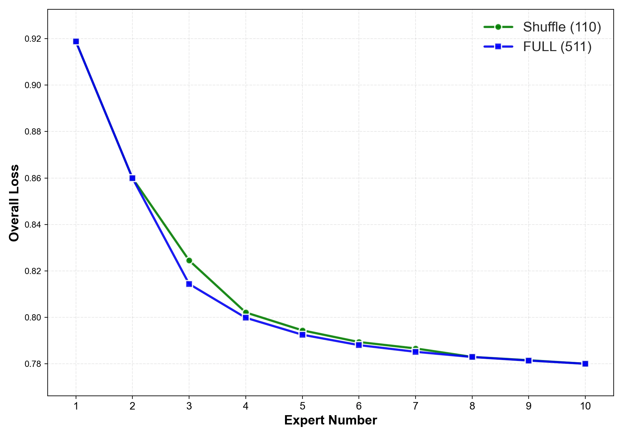
The sampled curves closely match full merging combinations on the 0.5B model.
Expert Post-Training Scaling
The paper also studies the scaling behavior of the domain expert models before merging. It relates expert loss to model size, training tokens, and compute budget. Larger models and larger post-training compute generally improve expert performance, consistent with standard language-model scaling laws.
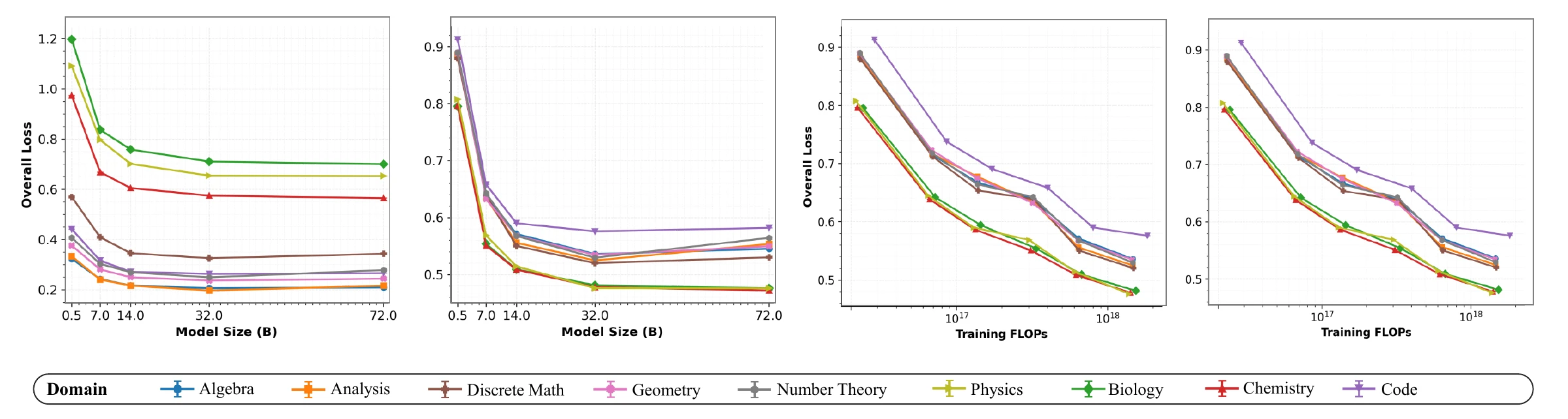
Expert post-training scaling: loss improves with model size and compute, but domains have different intrinsic loss levels.
The appendix highlights a domain-specific difference: Biology has substantially higher loss than Geometry under comparable training conditions, suggesting that different domains have different pre-existing knowledge reserves and may create heterogeneous merge dynamics.
Empirical Construction Details
The expected merge curve is built by plotting individual subset losses as light points and the per- mean as the fitted curve. As grows, individual losses still vary by subset, but the scatter narrows and the average remains smooth.


Representative empirical construction cases for Average and DARE at small and large base-model sizes.
In-Domain Fit Details
For each domain , the appendix fits:
The floor term is summarized as , and the tail as . Floors show tight power-law fits with exponents clustered around 0.33 to 0.42 and near 0.98 to 0.99. Tails are smaller and noisier, with Code showing the clearest decay with model size.
| Domain | ||||||||
|---|---|---|---|---|---|---|---|---|
| algebra | 0.000 | 0.0460 | -0.004 | -0.002 | 0.1724 | 0.1248 | 0.379 | 0.983 |
| analysis | 0.000 | 0.0462 | +0.009 | +0.009 | 0.1793 | 0.1255 | 0.417 | 0.990 |
| biology | 0.125 | 0.1741 | -0.006 | +0.007 | 0.6227 | 0.6338 | 0.362 | 0.988 |
| chemistry | 0.075 | 0.1317 | -0.006 | +0.008 | 0.4924 | 0.5639 | 0.331 | 0.988 |
| code | 0.250 | 0.0682 | +0.115 | 0.556 | 0.2705 | 0.2238 | 0.378 | 0.986 |
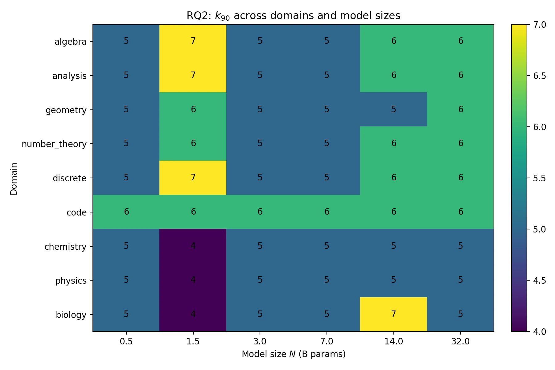
At under Average merging, macro CE decreases from 0.739 at 0.5B to 0.430 at 32B, a 41.9% reduction. The calculation illustrates why model size and tail amplitude should be considered separately: Code needs about eight experts at 0.5B and five experts at 32B for , while Biology has a nearly flat tail and needs roughly 18 experts despite the floor improving with .
Fractional Return and Expert Budget
The appendix computes the fraction of realized improvement:
using a monotone envelope of the measured CE curve. Median return reaches 85% at and 90% at , with concentrated in across domains and sizes.
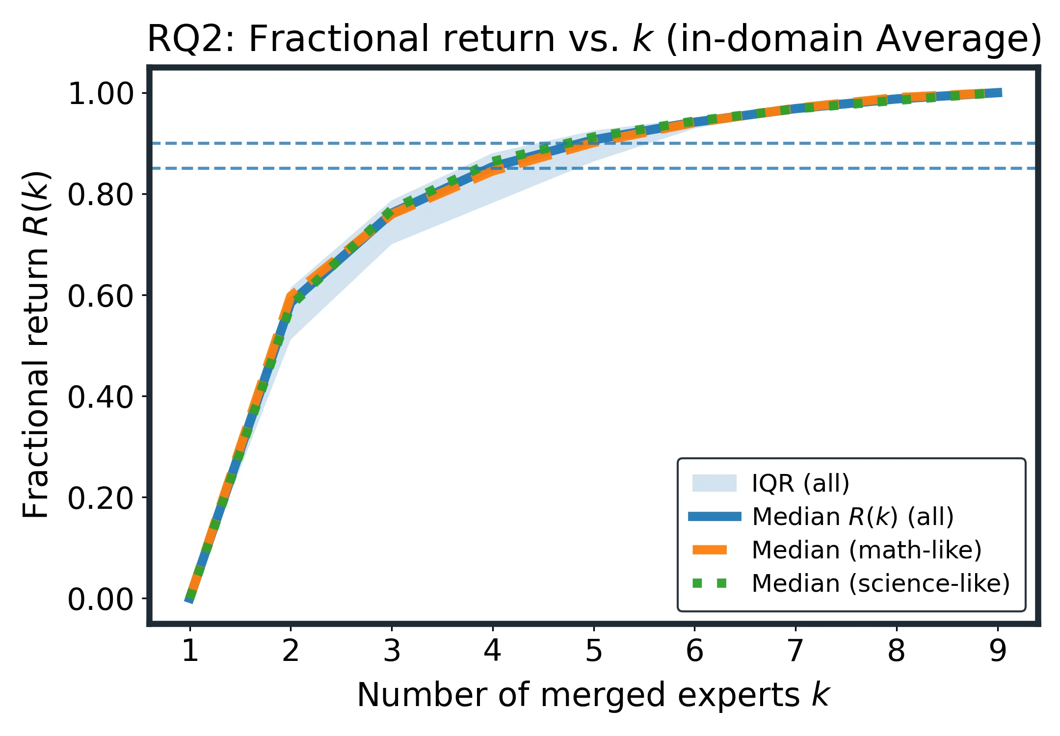
Most of the gain comes from the first few experts; k=6 recovers about 90% of the realized improvement.
The diminishing return follows from the floor-tail law: the marginal gain scales approximately as , so returns decay roughly as after the first few experts.
Cross-Domain Fit Details
The cross-domain appendix fits the same functional form to pooled CE and to method-specific curves. Average, TA, TIES, and DARE all follow:
For TIES, the appendix notes that the strongest nonlinear cases may be better captured with a small bounded interference term:
The reported headline pattern remains unchanged: most pooled improvement is achieved by , method differences narrow as increases, and scaling lowers both the floor and the tail.
The appendix also analyzes whether a larger candidate pool helps. With 7- and 8-domain pools, the fitted floor and tail remain stable and the qualitative law is unchanged.
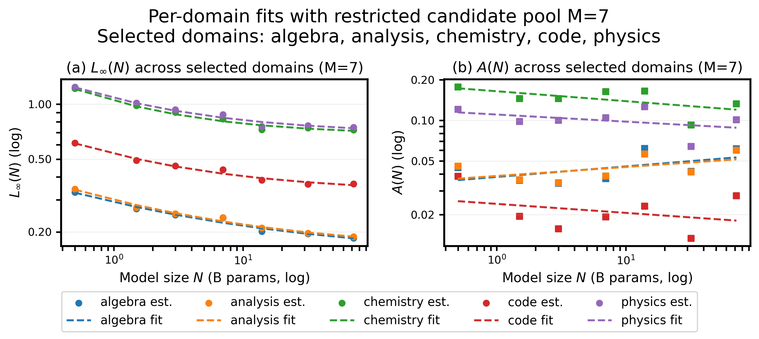
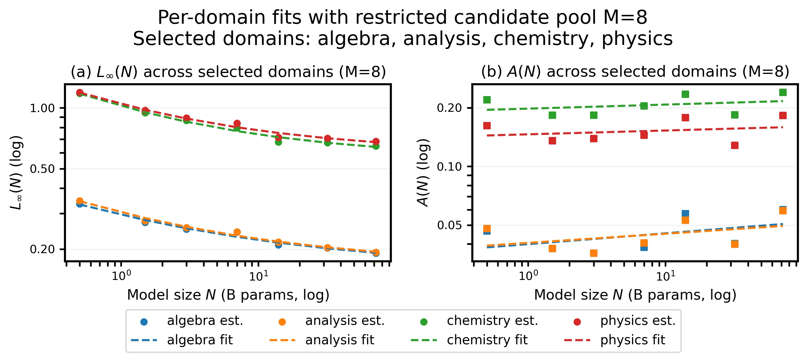
Candidate-pool variants keep the same floor-plus-tail behavior.
Downstream Metrics
To test whether CE trends transfer to task quality, the paper evaluates merged checkpoints on math, reasoning, multilingual, coding, and safety benchmarks. For each backbone and merge method, it evaluates all expert subsets for , normalizes metrics so larger is better, and reports mean accuracy averaged across benchmarks and subsets.
| Backbone | Method | |||||
|---|---|---|---|---|---|---|
| LLaMA-3.1 8B | TA | 0.411 | 0.443 | 0.456 | 0.462 | 0.469 |
| LLaMA-3.2 3B | TA | 0.375 | 0.386 | 0.388 | 0.389 | 0.388 |
| Gemma-2 2B | TA | 0.492 | 0.503 | 0.506 | 0.507 | 0.507 |
| LLaMA-3.1 8B | TIES | 0.388 | 0.414 | 0.426 | 0.436 | 0.436 |
The downstream trend mirrors the CE law: performance improves as more experts are merged, then saturates. LLaMA-3.1 8B with TA rises from 0.411 to 0.469 from to , while LLaMA-3.2 3B shows a shallower tail and small fluctuations near the plateau. The appendix attributes those fluctuations to benchmark variance rather than a systematic collapse.
The detailed downstream tables cover five specialized experts: math, code, multilingual, safety, and instruction following. Benchmarks include MATH-500, GSM8K, MBPP+, HumanEval+, IFEval, ARC, HellaSwag, MMLU, multilingual overall, and safety.
Scaling With 16 Domains
The appendix extends the cross-domain experiment to a 16-domain pool on the LLaMA3-3B-Instruct backbone. It starts with the original nine domains and adds Japanese, medical, house-arrangement, Korean, emotion, elementary school mathematics, and Java code.
For , the paper samples random TA merges and evaluates CE, variance, and standard deviation across subsets. The macro-average keeps the same pattern:
| Statistic | ||||||||
|---|---|---|---|---|---|---|---|---|
| Overall CE | 0.7774 | 0.7331 | 0.7051 | 0.6874 | 0.6685 | 0.6603 | 0.6509 | 0.6437 |
| Overall variance | 0.0009 | 0.0017 | 0.0021 | 0.0018 | 0.0012 | 0.0006 | 0.0024 | |
| Overall std | 0.0310 | 0.0418 | 0.0461 | 0.0424 | 0.0357 | 0.0251 | 0.0156 |
The larger domain pool does not change the qualitative behavior: CE drops as more experts are merged, gains flatten at larger , and subset variability generally contracts.
Cross-Domain Synergy
The paper measures donor-receiver interactions by adding one expert at a time and recording the marginal CE change on every evaluation domain. This yields a synergy matrix .
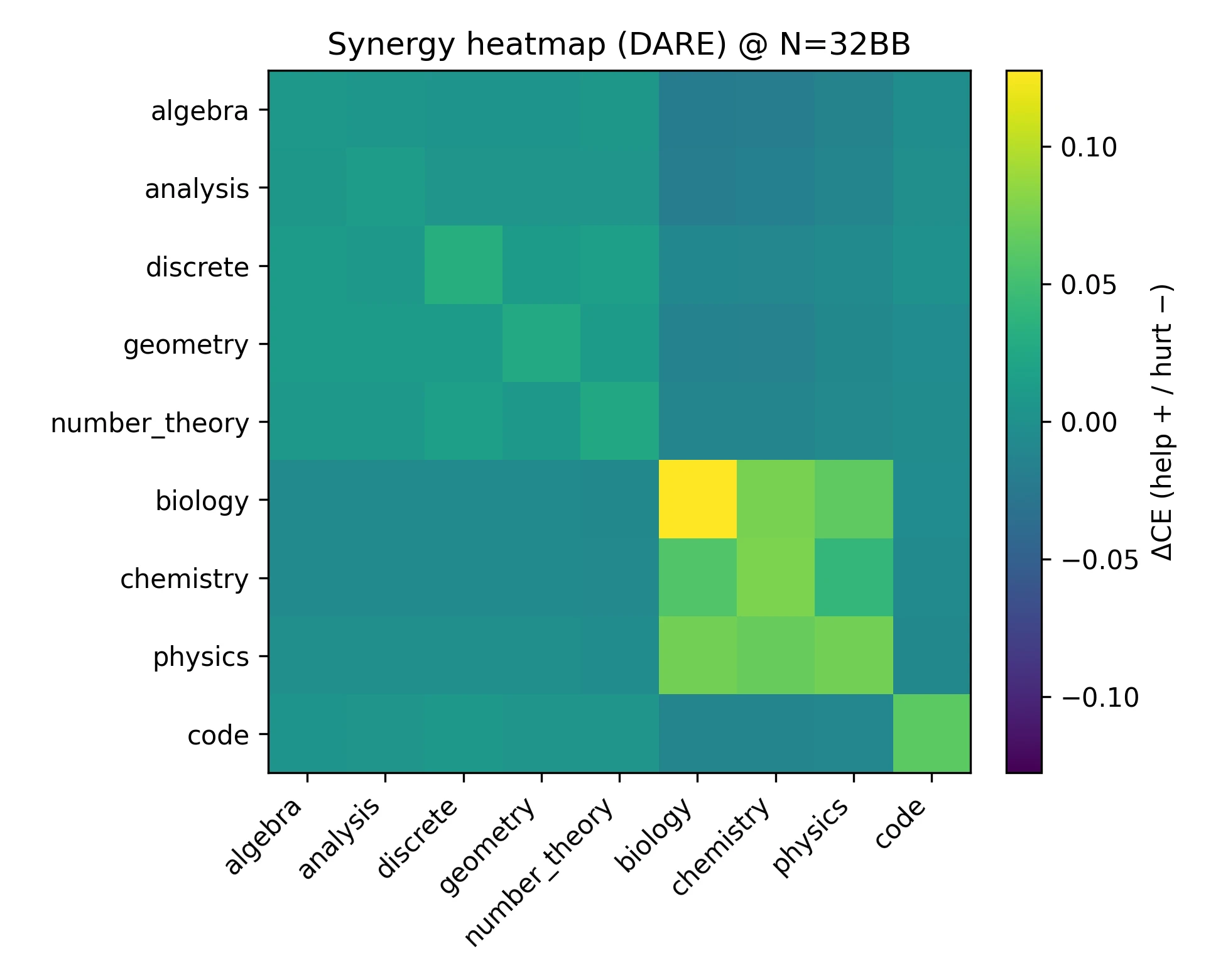
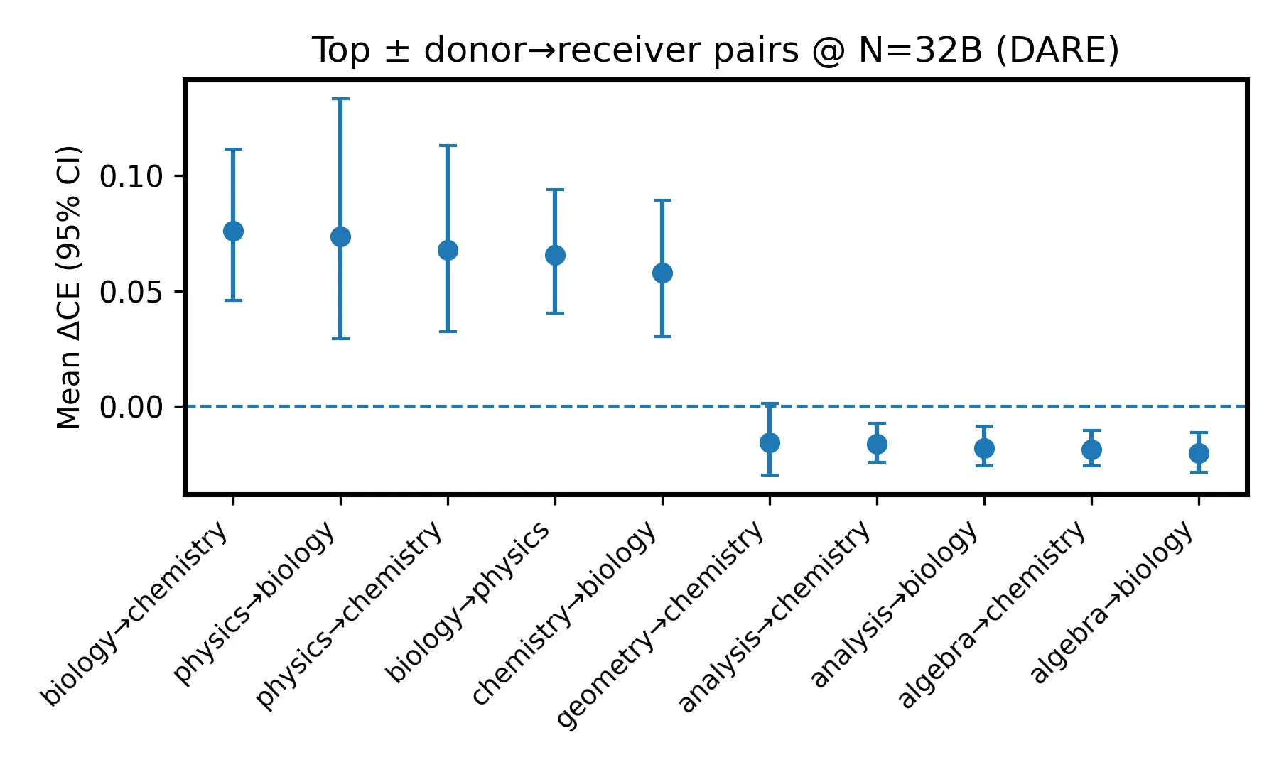
DARE at 32B shows structured synergy: science helps science, math helps math, and cross-block transfers are weaker or mildly negative.
Under DARE at 32B, science-to-science pairs are strongly positive, math-to-math pairs are moderately positive, and cross-block interactions are weakly negative. Code mildly helps Discrete and Geometry. The strongest off-diagonal positives are Biology to Chemistry (+0.076), Physics to Biology (+0.074), Physics to Chemistry (+0.068), Chemistry to Biology (+0.066), and Biology to Physics (+0.054). The largest negatives include Algebra to Physics (-0.026), Geometry to Chemistry (-0.020), Discrete to Chemistry (-0.018), Algebra to Biology (-0.016), and Number Theory to Biology (-0.015).
For practical selection, the appendix suggests prioritizing Physics, Biology, and Chemistry donors for science targets, and staying within the math block or including Code for math targets.
Additional Order and Backbone Details
Across-order dispersion is measured from DARE merge permutations. The paper fits:
Order sensitivity drops rapidly from to . For example, at 32B, mean CE changes from 0.5207 at to 0.4634 at , while across-order std drops from 0.0313 to 0.0060 and the range drops from 0.0865 to 0.0148.
On LLaMA backbones, the appendix fits:
| Backbone | ||||||
|---|---|---|---|---|---|---|
| LLaMA-3.2 3B | 0.9989 | 0.6875 | 0.7137 | 0.0783 | 0.7599 | 0.7221 |
| LLaMA-3 8B | 0.9955 | 0.0000 | 0.7252 | 0.0573 | 0.7837 | 0.7325 |
This supports the claim that the same inverse-tail law transfers beyond Qwen2.5.
Additional Method-Size Slices
The appendix includes method comparisons across several fixed expert counts. These show the same compression of method gaps as model size and expert count increase.
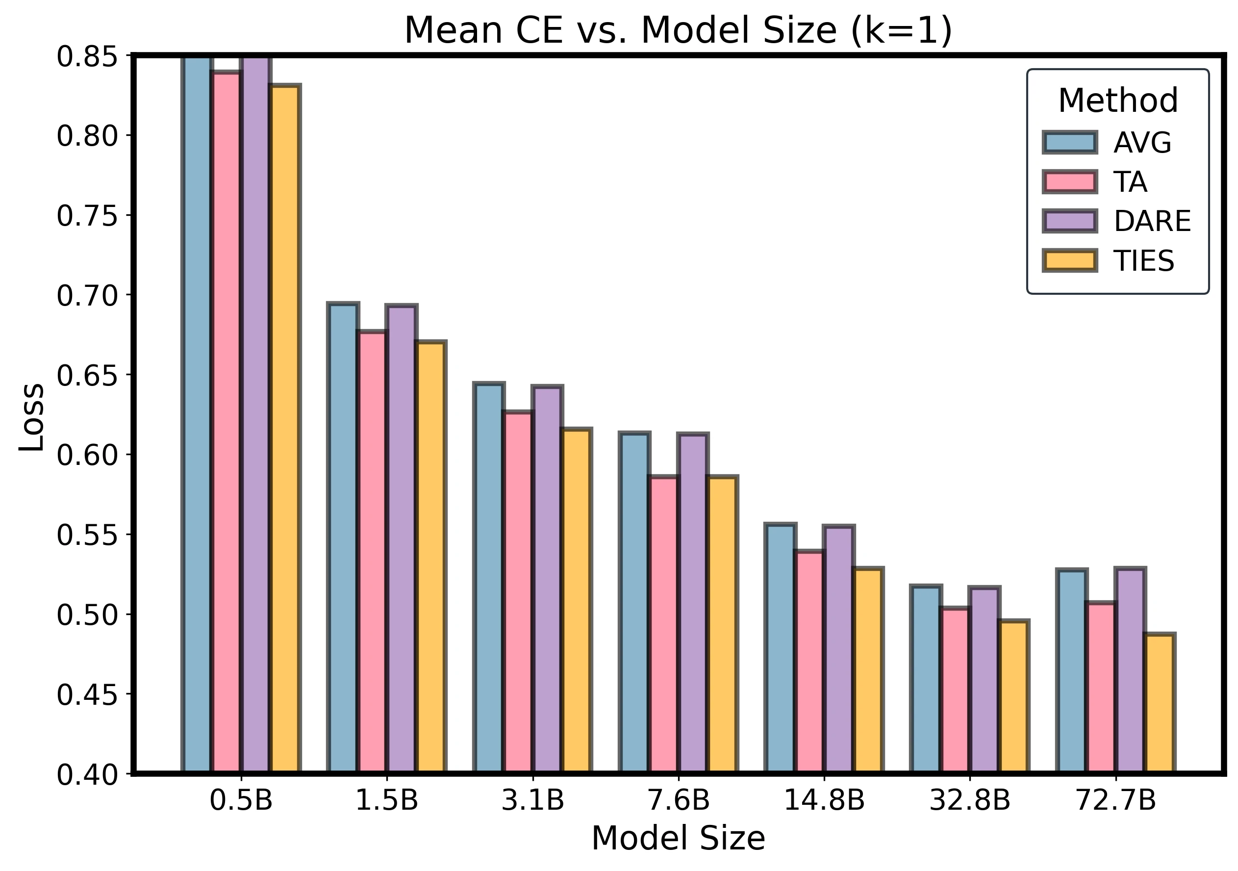
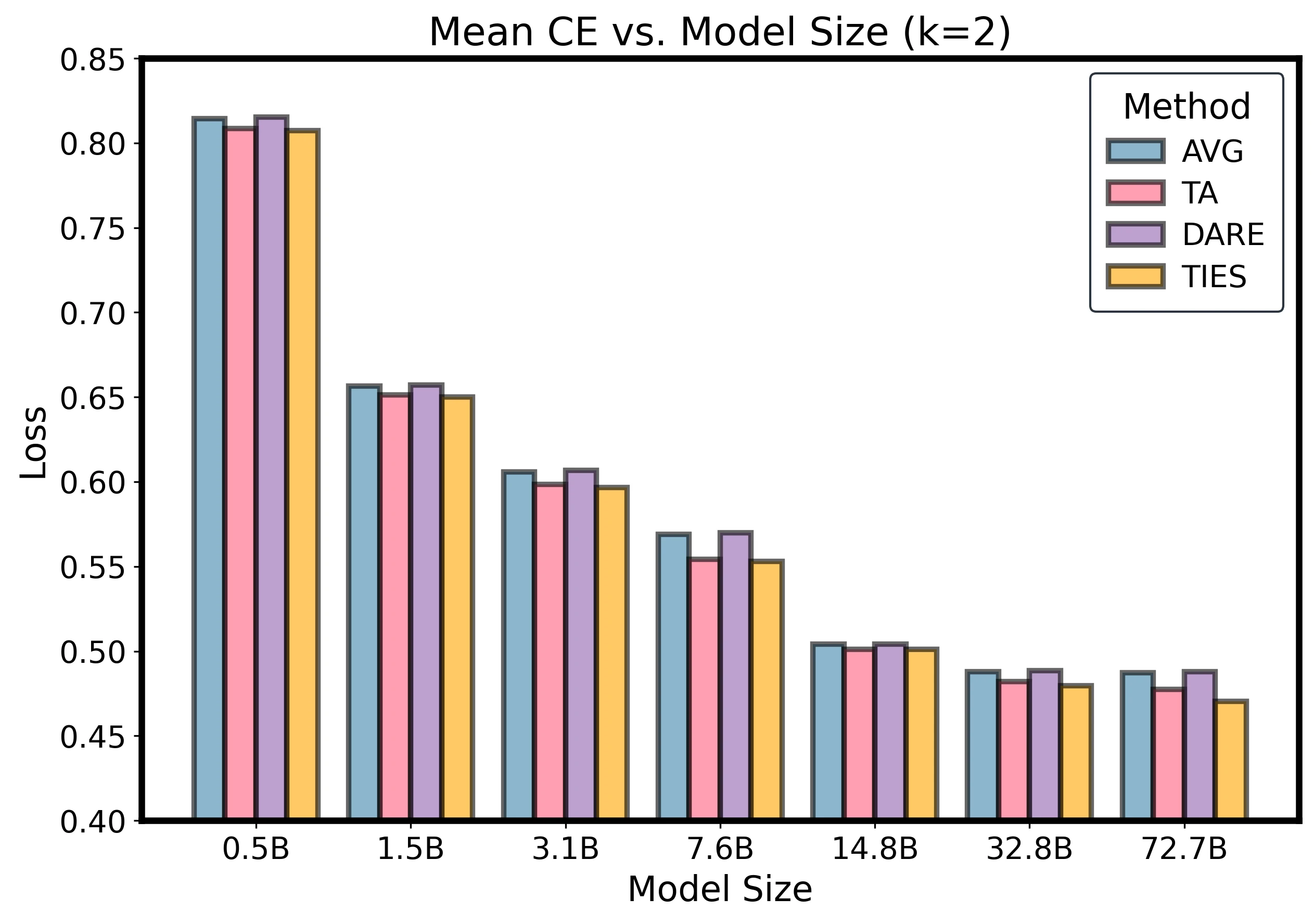
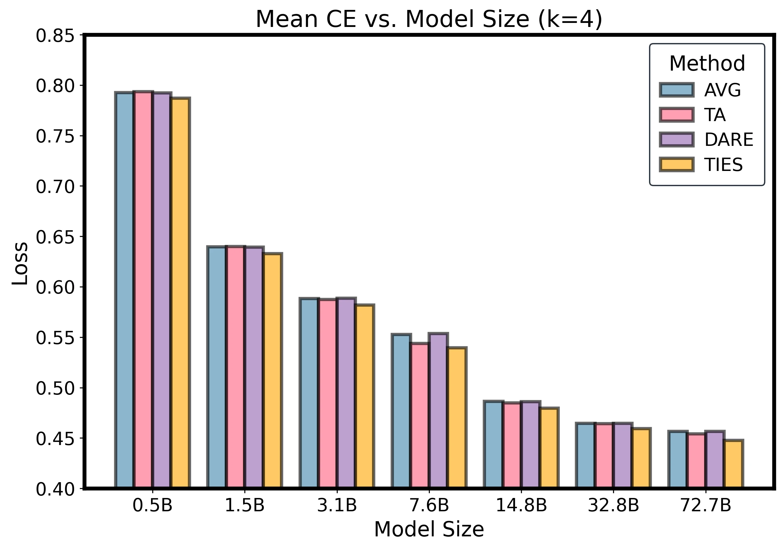
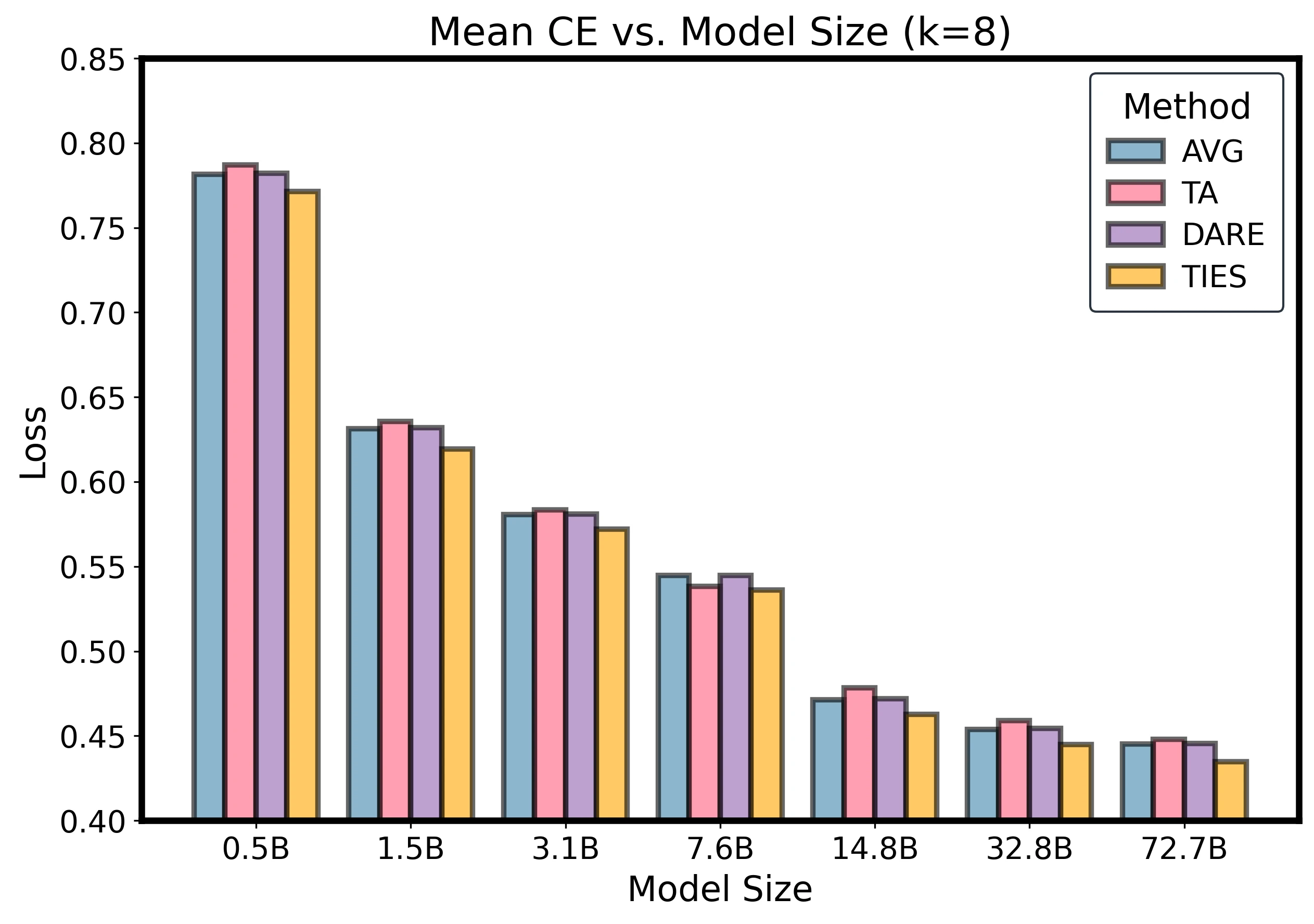
Method comparison slices at fixed k.
Impact Statement
This work advances understanding of model merging by characterizing how performance evolves with model size and expert count. By making expert merging more predictable, the scaling law can reduce unnecessary computation in large-scale model development. The techniques operate on trained models and do not introduce new objectives or data sources, so they inherit the same ethical considerations as existing LLMs.
More predictable merging may reduce the cost of deploying specialized capabilities, but it may also make powerful models more accessible. The paper does not identify negative ethical consequences unique to this method beyond those already associated with large-scale machine learning systems.
Limitations
The study centers on cross-entropy and equal-normalized composition. Extending the law to other objectives and adaptive weighting is an important next step.
The empirical evidence is broad across tested datasets, methods, and backbones, but it still does not cover extreme scales, additional modalities, or the full range of downstream metrics. Robustness, safety, and calibration remain open dimensions.
Expert capacity is controlled rather than treated as a third scaling axis. Changing LoRA rank, adapter width, training tokens, or expert quality should alter the effective-update statistics and therefore the fitted floor and tail parameters.
On the theoretical side, the paper leaves open a sharper connection between floor/tail parameters, curvature anisotropy, and domain dispersion. Better selection and ordering policies that exploit these quantities could tighten predictions and automate practical merging at scale.
BibTeX
@inproceedings{wang-2026-merging-scaling-law,
      title={Model Merging Scaling Laws in Large Language Models},
      author={Yuanyi Wang and Yanggan Gu and Yiming Zhang and Qi Zhou and Zhaoyi Yan and Congkai Xie and Xinyao Wang and Jianbo Yuan and Hongxia Yang},
      booktitle={Proceedings of the 43rd International Conference on Machine Learning},
      year={2026},
      url={https://github.com/InfiXAI/Merging-Scaling-Law},
}