FeatCal: Feature Calibration for Post-Merging Models
ABSTRACT
Model merging combines task experts into one model and avoids joint training, retraining, or deploying many expert models, but the merged model often still underperforms task experts. We study this performance gap through *feature drift*, the difference between features produced by the merged model and by the expert on the same input. Our theory decomposes this drift into upstream propagation and local mismatch, tracks how it propagates and combines through later layers in forward order, and links final feature drift to output drift. This view motivates FeatCal, which uses a small calibration set to calibrate the merged model weights layer by layer in forward order, reducing feature drift while staying close to merged weights and preserving the benefits of model merging. FeatCal uses an efficient closed-form solution to update model weights, with no gradient descent, iterative optimization, or extra modules. On the main CLIP and GLUE benchmarks, FeatCal beats Surgery and ProbSurgery, the closest post-merging calibration baselines: 85.5% vs. 77.0%/78.8% on CLIP-ViT-B/32 Task Arithmetic (TA) and 85.2% vs. 83.7%/82.2% on FLAN-T5-base GLUE. On CLIP-ViT-B/32, 8 examples per task reach 82.9%, and 256 examples per task take 53 seconds, about 4x faster than both baselines, showing better sample efficiency and lower calibration cost.
 May 13, 2026
 Yanggan Gu, Shuo Cai, Zihao Wang, Wenjun Wang, Yuanyi Wang, Pengkai Wang, Sirui Huang, Su Lu, Jianmin Wu, Hongxia Yang
Abstract
Model merging combines task experts into one model and avoids joint training, retraining, or deploying many expert models, but the merged model often still underperforms task experts. We study this performance gap through feature drift, the difference between features produced by the merged model and by the expert on the same input. Our theory decomposes this drift into upstream propagation and local mismatch, tracks how it propagates and combines through later layers in forward order, and links final feature drift to output drift. This view motivates FeatCal, which uses a small calibration set to calibrate the merged model weights layer by layer in forward order, reducing feature drift while staying close to merged weights and preserving the benefits of model merging. FeatCal uses an efficient closed-form solution to update model weights, with no gradient descent, iterative optimization, or extra modules. On the main CLIP and GLUE benchmarks, FeatCal beats Surgery and ProbSurgery, the closest post-merging calibration baselines: 85.5% vs. 77.0%/78.8% on CLIP-ViT-B/32 Task Arithmetic (TA) and 85.2% vs. 83.7%/82.2% on FLAN-T5-base GLUE. On CLIP-ViT-B/32, 8 examples per task reach 82.9%, and 256 examples per task take 53 seconds, about 4x faster than both baselines, showing better sample efficiency and lower calibration cost.
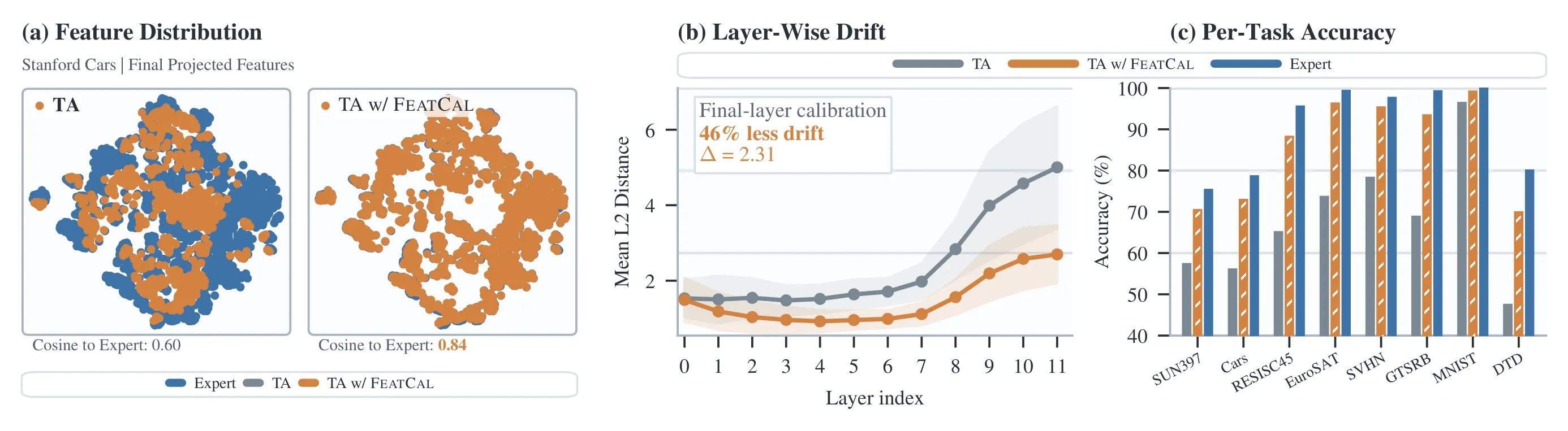
Figure 1. Feature drift after Task Arithmetic (TA) merging and FeatCal calibration in CLIP-ViT-B/32. Panels (a,b) use Stanford Cars: FeatCal moves features toward expert features, raises their mean cosine similarity from 0.60 to 0.84, and reduces mean L2 feature drift, with 46% less final-layer drift. Panel (c) reports per-task accuracy in the 8-task setting. Appendix B gives full 8-task feature views.
1. Introduction
Model merging composes task experts into one model, avoiding joint training, retraining, or deploying a separate model for each task. However, the merged model often still underperforms the experts it is intended to combine. This leaves a clear performance gap after merging in practice.
We analyze this gap through feature drift, the difference between features of the merged model and the task expert on the same input sample. Our layer by layer analysis decomposes this drift into upstream propagation and local mismatch at expert input features, then shows how local mismatches propagate through later layers in forward order and combine into final feature drift. We further analyze how final feature drift reaches the model output and becomes output drift, explaining how feature drift can affect output scores. Figure 1 illustrates this behavior on CLIP-ViT-B/32 merged with Task Arithmetic (TA), where final features move away from the Stanford Cars expert features and drift appears across multiple layers of the network after TA merging.
Surgery and ProbSurgery are related post-merging calibration methods: they identify feature drift at the final layer and train extra modules for calibration. Other intervention methods point to the same lesson: expert signals can help, but current methods often rely on task specific intervention parameters, extra modules at inference, or iterative optimization. These choices make calibration less direct for an already merged model and can leave the final model with an auxiliary inference path. This motivates efficient, direct calibration that preserves inference speed.
FeatCal uses our drift analysis as a design cue for calibrating the merged model. It uses a forward-order schedule suggested by the propagation view and calibrates the model layer by layer. We introduce a regularization term that keeps the calibrated model close to the merged model, which helps preserve the benefits of model merging and reduce overfitting to the small calibration set. The resulting objective has an efficient closed form solution, so calibration needs no gradient descent, iterative optimization, or extra modules at inference. We further introduce feature interpolation and anchor regularization to balance expert signals with the merged model and improve performance.
Empirically, Figure 1 shows the practical effect: FeatCal moves merged features toward expert features, reduces feature drift, and raises per-task accuracy after TA merging. On CLIP-ViT-B/32 8-task TA, it reaches 85.5% versus 77.0%/78.8% for Surgery/ProbSurgery, and on FLAN-T5-base GLUE it reaches 85.2% versus 83.7%/82.2%. The same trend holds on CLIP-ViT-L/14 WUDI, FLAN-T5-large, and MergeBench Llama-family LLM merging, where FeatCal improves TA by / average points on 3B/8B models. On CLIP-ViT-B/32 TA, 8 examples per task reach 82.9%, and calibration with 256 examples per task takes 53 seconds, about 4x faster than both baselines under the same calibration protocol.
We summarize the main contributions of this work as follows: ① We develop a theory of feature drift after merging, with an exact decomposition into local mismatch and upstream propagation, forward order propagation, and a link to output drift. ② We introduce FeatCal, which efficiently calibrates merged model weights in forward order with closed form updates, without gradient descent, architecture changes, or extra modules at inference. ③ We validate FeatCal on CLIP, FLAN-T5, and MergeBench LLM benchmarks, where it outperforms related post-merging calibration baselines while using fewer samples and lower calibration cost without adding inference-time modules.
2. Related Work
Model Merging. Most model merging methods build a fused model by merging task experts directly in parameter space. Methods based on feature statistics or feature drift, such as RegMean, RegMean++, and LOT Merging, are closer in mechanism: they derive layer updates during merging from feature statistics, regression objectives, or an explicit feature drift objective. These methods define how to build the merged model. In contrast, FeatCal treats that model as the starting point, uses a small calibration set and task experts for post-merging calibration, and controls calibration strength through regularization. This stage separation matters because calibration must work with the feature drift left by a chosen merger instead of changing the merge rule itself. It helps preserve the benefits of model merging while reducing the risk of overfitting to calibration data.
Post-Merging Feature Calibration. Representation Surgery and follow-up methods operate on merged-model features through task-specific plugins, deeper interventions, probabilistic feature-drift modeling, or parameter-efficient modules. These closest post-merging alternatives establish that expert-guided feature calibration is useful. FeatCal differs in parameterization and deployment: instead of learning or deploying auxiliary intervention modules, it folds the calibration into the original linear module weights through closed-form regularized updates, leaving a single architecture-preserving model at inference time rather than an auxiliary intervention path.
3. Post-Merging Feature Drift: Problem Formulation and Properties
Before introducing FeatCal, we formalize post-merging feature drift and show how local mismatch is defined at expert input features, then propagated and combined in forward order across depth.
3.1 Layer-Wise Feature Drift
We consider task experts and a merged model . As in standard weight-space merging, experts are fine-tuned from a common pretrained base. All models share the same architecture and contain layers. Let be the data distribution of task . For layer , and denote the corresponding layer functions of the task expert and the merged model, respectively.
For an input sample from task , define the expert and merged layer output features recursively as
Definition 1. [Layer-wise feature drift]
For task , sample , and layer , the layer-wise feature drift is the difference between the merged-model feature and the corresponding task-expert feature at that layer:
This pointwise drift signal is the object propagated in forward order in the analysis below.
3.2 Local Mismatch and Drift Propagation
Proposition 1. [Exact layer-wise drift decomposition]
For every task , sample , and intermediate layer , the drift decomposes as follows. By Eq. 1, .
Proof. The algebraic identity and its regularity details are deferred to Appendix C.
Interpretation. Proposition 1 decomposes layer-wise feature drift into two terms: local mismatch and upstream-drift propagation. The local mismatch measures the feature mismatch caused by the difference between the merged and expert layer maps at the same expert input feature. The propagation term measures how feature drift inherited from earlier layers changes the input feature of layer and is then carried into the output feature of this layer.
Proposition 2. [Layer-wise propagation of local mismatch]
Fix a task , sample , and layers . Suppose that, for each layer , is continuously differentiable on an open neighborhood containing the segment between and . Let denote the corresponding path-averaged local sensitivity operator, defined explicitly in Eq. 18. Then the drift obeys the layer-by-layer recursion
Since , the final feature drift is
The product composes compatible local maps. See Eq. 21 for the -to- form.
Proof. The local sensitivity derivation and unrolled expansion are deferred to Appendix C.
Interpretation. Proposition 2 gives a simple forward-order view: local mismatches arise at individual layers, and their induced feature drift propagates through downstream layers to the final layer. Thus, final feature drift is a downstream combination of local mismatches from different layers. For residual networks, we further show that residual paths carry upstream feature drift through the skip connection. The drift can also grow under specific conditions. See Appendix D.
3.3 From Feature Drift to Output Drift
Definition 2. [Output drift for task scores]
For the merged model , let and be the expert and merged task scores, each represented as a score vector. Let and map final features to task scores, with and . The post-merging output drift is
In the logit or similarity settings used below, can contain class logits, CLIP candidate scores (scaled similarity scores over a fixed candidate set), or fixed-prefix decoder vocabulary logits.
Proposition 3. [Feature-to-output perturbation]
Suppose is locally -Lipschitz on the segment between and . Here locally bounds how much the merged task score map can change when its final-feature input moves along this segment. Then
where
is the score map mismatch. If the task score map is shared, this term is .
Proof. This is the perturbation bound proved in Proposition 6.
Interpretation. Proposition 3 shows that final feature drift can propagate to output drift, thus further affect model outputs and task loss. For example, in a language model under a fixed prefix, token probabilities are obtained by applying softmax to output logits. Holding other logits fixed, a larger token logit gives a larger token probability, so output-logit drift can potentially induce probability drift and change the next-token choice. Cross-entropy loss is also tied to the probability assigned to the target token, so probability drift can induce loss drift. Detailed analysis is deferred to Appendix E.
4. FeatCal: Feature Calibration for Post-Merging Models
The preceding drift analysis guides the design of a direct calibration procedure for an already merged model. FeatCal visits layers in forward order, takes a current feature snapshot after earlier layer updates, and solves expert-guided calibration objectives for the modules in that layer with explicit regularization.
4.1 Basic Calibration Objective
Forward-order calibration. The drift analysis in Section 3.2 shows that feature drift arises from local mismatch terms that propagate layer by layer in forward order. FeatCal follows the same order by calibrating the merged model layer by layer: after earlier layers are calibrated, it recollects current calibrated-model features for the next layer before fitting that layer's module objectives. This schedule also reduces mismatch between features used during calibration and features exposed by the deployed calibrated model; Appendix F formalizes this source/deployed feature mismatch.
Why calibrate linear modules? Under this schedule, each layer provides a shared feature snapshot. Given the cached input features and expert target features for a module in that snapshot, the local surrogate can be defined for any linear module. In practice, FeatCal applies it to the modules configured for calibration. Linear modules are natural feature-mixing and projection points in the architectures we study, including attention and MLP linear modules. Once their calibrated-model input features are fixed, each linear module gives a tractable regularized regression problem with a closed-form update. The update replaces the existing merged weight, preserving the architecture without gradient descent, adapters, or inference-time modules. For other affine components, including bias parameters and LayerNorm affine parameters, we also design calibration updates, as detailed in Appendix G. In practice, these extra updates give limited gains: on CLIP, their average accuracy improvement is less than 0.5 percentage points. The main gains come from calibrating linear modules.
Linear module feature drift. For a fixed linear module inside the current layer, we define a module-local version of feature drift using the variables available at that module. Let be the task- expert, merged, and base weights for this module. When processing the layer, we cache fixed input feature matrices and for this module on the same task- calibration samples. Here is produced by the prefix-calibrated model and is therefore the deployed input source, while is the corresponding task-expert feature matrix.
Following the layer-wise feature drift definition in Eq. 2, we define the linear module feature drift of a candidate calibrated weight by
As in the layer-wise analysis, this module-level drift can be interpreted as a combination of module-local mismatch and upstream-drift propagation.
Basic calibration objective. With input features fixed, the per-module calibration objective minimizes the overall linear module feature-drift error with a merged-weight penalty:
The quadratic penalty controls how far a single module update can move from the merged weights. This objective is a tractable module-local surrogate for reducing linear module feature drift, rather than an exact objective for end-to-end task risk or all-layer feature drift.
4.2 Feature Interpolation for Calibration Targets
Under the forward-order schedule, each layer's calibration should focus on the local mismatch at its current linear module rather than compensate for feature drift caused by upstream layers. Directly using expert input features for calibration can violate this goal. The gap between and already contains upstream feature drift, so fitting the direct target may force the current linear module to fit drift left by earlier layers. We therefore introduce an interpolated target feature:
In Eq. 9, we replace the target term with . This target keeps the expert signal while making the local regression less aggressive under upstream drift.
4.3 Anchor Regularization
During calibration, the objective should use targets formed from expert features while keeping the update tied to the merged weights. The base model provides another useful reference. It is pretrained on large data before task specialization and can contain knowledge that a small calibration set does not cover. To use this reference, we include the base weight in the regularization term. The coefficients below let us control how calibration uses the merged and base references. For a linear module, we define the anchor weight as
The coefficient controls the anchor used by the quadratic penalty.
Combining the target interpolation in Eq. 10 and the anchor in Eq. 11 gives the practical objective:
The first term uses the interpolated target from Eq. 10 to fit the expert feature signal without using the raw expert input feature as a hard target. The second term uses the anchor from Eq. 11 to keep the update close to the chosen reference, with controlling the regularization strength.
4.4 Task-Wise Scale Normalization and Closed-Form Solution
This subsection describes the update applied after feature collection. At each forward-order layer, FeatCal first caches current calibrated-model features and expert features for the modules calibrated in that layer. The cached features are then used to compute each linear module update separately, and the layer parameters are loaded after the layer's updates are formed. Thus the statistics below are module-local, even though feature collection is organized by layer.
For a fixed linear module in the current layer, let denote the calibration sample count for each task at this module. The factors form per-task empirical moments and prevent each task contribution from scaling directly with the sample count. We summarize task by the empirical feature statistics
Here, is the input second moment and is the target-input cross moment.
The objective in Eq. 12 is a matrix-valued ridge regression problem. To reduce scale sensitivity, we use stabilized inverse task weights with ,
With these stabilized task weights fixed, the module-wise objective becomes
The corresponding stationary condition for this quadratic objective is
Solving this linear system gives the closed-form update for this module
Because , , and , the inverse is well defined. In implementation, we also add to the solve matrix as a numerical stabilizer.
The complete forward-order calibration procedure is given in Appendix H.
5. Experiments
5.1 Setup
Benchmarks. We use two public FusionBench settings and one MergeBench LLM setting : ① CLIP image classification. We use the FusionBench CLIP model merging benchmark with CLIP-ViT-B/32 and CLIP-ViT-L/14. The primary setting has 8 image tasks: SUN397, Stanford Cars, RESISC45, EuroSAT, SVHN, GTSRB, MNIST, and DTD. The 14-task suite adds Flowers102, PCAM, FER2013, Oxford-IIIT Pet, STL10, and CIFAR100. The 20-task suite further adds CIFAR10, Food101, Fashion-MNIST, EMNIST Letters, KMNIST, and Rendered SST2. We follow prior merging protocols, report top-1 accuracy and task averages, and defer full per-task extended results to Appendix I. ② FLAN-T5 text generation. We evaluate FusionBench FLAN-T5-base and FLAN-T5-large merging on 8 prompted GLUE tasks: CoLA, MNLI, MRPC, QNLI, QQP, RTE, SST-2, and STS-B. The base experts are full fine-tuned models, while the large experts use LoRA fine-tuning. We merge task experts and evaluate generated text outputs. We report exact match accuracy except for STS-B, where we report Spearman's , and average the 8 task scores. ③ MergeBench LLM merging. We evaluate Llama-3.2-3B-Instruct and Llama-3.1-8B-Instruct in the MergeBench domain-expert setting. The task suite covers mathematics, coding, instruction following, and general knowledge through MATH-500, GSM8K, HumanEval+, MBPP+, IFEval, and ARC-Challenge. HumanEval+ and MBPP+ report pass@1, and each table average is the mean over all 6 reported MergeBench tasks in this LLM setting.
Compared methods. We compare against pre-trained, single-task, and multi-task references when available. For CLIP, upstream mergers include Simple Averaging, Task Arithmetic, AdaMerging, and WUDI-Merging; for FLAN-T5 and MergeBench, we use Task Arithmetic. We apply FeatCal on top of different upstream mergers and compare with Surgery and ProbSurgery where available. Unless otherwise stated, upstream and baseline hyperparameters follow the FusionBench recipes.
Calibration setup. By default, FeatCal uses 256 calibration samples per task, calibrates layers in forward order, and applies the linear-weight update in Eq. 17. When enabled, it also applies the bias and LayerNorm affine updates in Appendix G; the main CLIP runs enable both, while the FLAN-T5 runs calibrate linear-module bias parameters but not LayerNorm affine parameters. For the main CLIP accuracy tables, we fix , , and . For FLAN-T5, we use , , and . For MergeBench, we use for Llama-3.2-3B-Instruct and for Llama-3.1-8B-Instruct. Test sets are used only for final reporting. Section 5.5 includes a compact sensitivity diagnostic for the 8-task TA setting.
5.2 Results on CLIP Models
Table 1. Multi-task performance of CLIP-ViT-B/32 models on 8 image-classification tasks. All numbers are top-1 accuracy (%). Gray arrows show changes over upstream mergers.
| Method | SUN397 | Cars | RESISC45 | EuroSAT | SVHN | GTSRB | MNIST | DTD | Avg. |
|---|---|---|---|---|---|---|---|---|---|
| Pre-trained | 63.2 | 59.8 | 60.7 | 46.0 | 31.6 | 32.5 | 48.2 | 43.9 | 48.2 |
| Fine-tuned (STL) | 75.0 | 78.3 | 95.2 | 99.0 | 97.3 | 98.9 | 99.6 | 79.7 | 90.3 |
| Traditional MTL | 72.3 | 76.6 | 92.2 | 97.9 | 95.5 | 97.7 | 99.3 | 77.7 | 88.6 |
| Simple Averaging | 65.4↑0.0 | 62.4↑0.0 | 70.6↑0.0 | 75.7↑0.0 | 64.5↑0.0 | 55.0↑0.0 | 86.3↑0.0 | 50.6↑0.0 | 66.3↑0.0 |
| w/ Surgery | 67.4↑2.0 | 63.5↑1.1 | 80.5↑9.9 | 94.7↑19. | 70.8↑6.3 | 79.7↑24. | 96.8↑10. | 64.7↑14. | 77.3↑11. |
| w/ ProbSurgery | 69.2↑3.8 | 65.8↑3.4 | 85.8↑15. | 93.4↑17. | 70.4↑5.9 | 87.0↑32. | 96.5↑10. | 69.1↑18. | 79.7↑13. |
| w/ FeatCal | 69.7↑4.3 | 70.4↑8.0 | 85.0↑14. | 95.4↑19. | 92.6↑28. | 87.1↑32. | 97.9↑11. | 67.4↑16. | 83.2↑16. |
| Task Arithmetic | 57.0↑0.0 | 55.7↑0.0 | 64.7↑0.0 | 73.3↑0.0 | 77.9↑0.0 | 68.5↑0.0 | 96.1↑0.0 | 47.1↑0.0 | 67.5↑0.0 |
| w/ Surgery | 59.9↑2.9 | 59.9↑4.2 | 76.1↑11. | 92.4↑19. | 83.6↑5.7 | 84.9↑16. | 98.0↑1.9 | 61.1↑14. | 77.0↑9.5 |
| w/ ProbSurgery | 60.6↑3.6 | 61.1↑5.4 | 81.0↑16. | 93.8↑20. | 85.3↑7.4 | 87.1↑18. | 97.9↑1.8 | 63.8↑16. | 78.8↑11. |
| w/ FeatCal | 70.1↑13. | 72.5↑16. | 88.1↑23. | 96.3↑23. | 95.0↑17. | 93.0↑24. | 98.8↑2.7 | 69.8↑22. | 85.5↑18. |
| AdaMerging | 67.9↑0.0 | 71.2↑0.0 | 84.0↑0.0 | 92.3↑0.0 | 87.6↑0.0 | 93.1↑0.0 | 98.2↑0.0 | 66.9↑0.0 | 82.7↑0.0 |
| w/ Surgery | 69.8↑1.9 | 72.1↑0.9 | 88.7↑4.7 | 95.3↑3.0 | 90.5↑2.9 | 95.7↑2.6 | 98.7↑0.5 | 73.3↑6.4 | 85.5↑2.8 |
| w/ ProbSurgery | 70.6↑2.7 | 72.9↑1.7 | 90.4↑6.4 | 95.8↑3.5 | 90.2↑2.6 | 95.0↑1.9 | 98.8↑0.6 | 73.8↑6.9 | 85.9↑3.2 |
| w/ FeatCal | 73.0↑5.1 | 77.4↑6.2 | 91.3↑7.3 | 96.8↑4.5 | 94.2↑6.6 | 96.7↑3.6 | 99.0↑0.8 | 76.4↑9.5 | 88.1↑5.4 |
| WUDI-Merging | 68.0↑0.0 | 72.5↑0.0 | 85.0↑0.0 | 94.6↑0.0 | 94.8↑0.0 | 95.0↑0.0 | 99.3↑0.0 | 66.7↑0.0 | 84.5↑0.0 |
| w/ Surgery | 69.0↑1.0 | 71.7↓0.8 | 89.1↑4.1 | 97.2↑2.6 | 95.6↑0.8 | 96.7↑1.7 | 99.3↑0.0 | 72.7↑6.0 | 86.4↑1.9 |
| w/ ProbSurgery | 69.5↑1.5 | 72.7↑0.2 | 90.6↑5.6 | 97.3↑2.7 | 95.6↑0.8 | 97.1↑2.1 | 99.3↑0.0 | 73.3↑6.6 | 86.9↑2.4 |
| w/ FeatCal | 72.2↑4.2 | 76.0↑3.5 | 93.0↑8.0 | 98.1↑3.5 | 96.7↑1.9 | 97.9↑2.9 | 99.4↑0.1 | 77.1↑10. | 88.8↑4.3 |
Table 2. CLIP Extended Average Accuracy.
| 2*Method | 8-Task | 14-Task | 14-Task | 20-Task | 20-Task |
|---|---|---|---|---|---|
| L/14 | B/32 | L/14 | B/32 | L/14 | |
| Pre-trained | 64.6 | 58.8 | 69.1 | 55.6 | 65.6 |
| Fine-tuned (STL) | 94.3 | 90.0 | 92.8 | 90.3 | 93.1 |
| Task Arithmetic | 80.5↑0.0 | 66.2↑0.0 | 77.3↑0.0 | 60.6↑0.0 | 70.3↑0.0 |
| w/ Surgery | 86.0↑5.5 | 76.8↑10. | 83.8↑6.5 | 75.2↑14. | 82.4↑12. |
| w/ ProbSurgery | 87.6↑7.1 | 78.3↑12. | 86.1↑8.8 | 77.7↑17. | 83.3↑13. |
| w/ FeatCal | 91.6↑11. | 81.5↑15. | 90.7↑13. | 79.4↑18. | 84.7↑14. |
| WUDI-Merging | 92.2↑0.0 | 78.7↑0.0 | 88.8↑0.0 | 67.1↑0.0 | 75.8↑0.0 |
| w/ Surgery | 92.8↑0.6 | 82.5↑3.8 | 90.3↑1.5 | 76.5↑9.4 | 84.9↑9.1 |
| w/ ProbSurgery | 93.0↑0.8 | 82.7↑4.0 | 90.7↑1.9 | 77.6↑10. | 86.5↑10. |
| w/ FeatCal | 93.5↑1.3 | 86.2↑7.5 | 91.5↑2.7 | 83.5↑16. | 89.8↑14. |
On B/32 8-task CLIP, FeatCal raises the 4 upstream averages from 66.3/67.5/82.7/84.5 to 83.2/85.5/88.1/88.8, beating Surgery and ProbSurgery in each block. The gains are largest for the weaker upstream mergers, but FeatCal also improves AdaMerging and WUDI-Merging, where the merged models are already close to the multi-task reference. This pattern aligns with the feature drift motivation: the same calibration step can recover large lost accuracy and still refine strong merged models without changing the merger itself. The best average, 88.8, is close to the 90.3 task expert average and above the 88.6 multi-task reference. For the TA and WUDI rows in Table 2, FeatCal remains above Surgery and ProbSurgery across all extended averages. On 20-task TA, FeatCal reaches 79.4 on B/32 and 84.7 on L/14, giving and points over TA. Full per-task results are in Appendix I.
5.3 Results on FLAN-T5 Models
Table 3. FLAN-T5 GLUE generation results. Scores are percentages: exact-match accuracy except STS-B, which reports Spearman's ; arrows show changes over Task Arithmetic, and bold marks best non-reference entries.
| 2*Model | 2*Method | GLUE Tasks | 2*Avg. | ||||||||
|---|---|---|---|---|---|---|---|---|---|---|---|
| CoLA | MNLI | MRPC | QNLI | QQP | RTE | SST-2 | STS-B | ||||
| Pre-trained | 69.1 | 56.5 | 76.2 | 88.4 | 82.1 | 80.1 | 91.2 | 62.2 | 75.7 | ||
| Fine-tuned (STL) | 75.0 | 83.4 | 87.5 | 91.5 | 85.4 | 85.9 | 93.6 | 88.7 | 86.4 | ||
| Task Arithmetic | 70.5↑0.0 | 57.8↑0.0 | 78.4↑0.0 | 90.2↑0.0 | 83.6↑0.0 | 80.5↑0.0 | 92.3↑0.0 | 77.8↑0.0 | 78.9↑0.0 | ||
| w/ Surgery | 70.8↑0.3 | 82.4↑24. | 82.4↑4.0 | 89.8↓0.4 | 84.2↑0.6 | 83.0↑2.5 | 92.1↓0.2 | 85.2↑7.4 | 83.7↑4.8 | ||
| w/ ProbSurgery | 82.4↑11. | 69.1↑11. | 78.3↓0.1 | 80.6↓9.6 | 89.8↑6.2 | 83.4↑2.9 | 81.2↓11. | 92.5↑14. | 82.2↑3.3 | ||
| w/ FeatCal | 72.2↑1.7 | 82.6↑24. | 85.1↑6.7 | 91.1↑0.9 | 84.7↑1.1 | 85.2↑4.7 | 93.0↑0.7 | 87.7↑9.9 | 85.2↑6.3 | ||
| Pre-trained | 73.7 | 56.6 | 82.4 | 91.1 | 85.5 | 85.6 | 94.3 | 87.5 | 82.1 | ||
| Fine-tuned (STL) | 80.2 | 88.5 | 89.2 | 94.4 | 87.2 | 91.7 | 95.2 | 90.9 | 89.6 | ||
| Task Arithmetic | 76.8↑0.0 | 85.4↑0.0 | 85.3↑0.0 | 94.0↑0.0 | 85.8↑0.0 | 88.1↑0.0 | 95.2↑0.0 | 87.7↑0.0 | 87.3↑0.0 | ||
| w/ Surgery | 76.0↓0.8 | 87.9↑2.5 | 86.0↑0.7 | 93.9↓0.1 | 86.2↑0.4 | 89.9↑1.8 | 95.2↑0.0 | 89.0↑1.3 | 88.0↑0.7 | ||
| w/ ProbSurgery | 77.2↑0.4 | 87.6↑2.2 | 85.0↓0.3 | 93.8↓0.2 | 86.0↑0.2 | 88.4↑0.3 | 95.2↑0.0 | 87.8↑0.1 | 87.6↑0.3 | ||
| w/ FeatCal | 79.2↑2.4 | 87.8↑2.4 | 89.0↑3.7 | 93.9↓0.1 | 86.9↑1.1 | 88.4↑0.3 | 95.3↑0.1 | 90.8↑3.1 | 88.9↑1.6 |
Table 3 shows that the GLUE gains hold for both FLAN-T5-base and FLAN-T5-large. For base, FeatCal improves Task Arithmetic by average points, exceeds Surgery and ProbSurgery, and improves all 8 tasks, with the largest gains on MNLI and STS-B. For large, where LoRA-based Task Arithmetic is already strong, FeatCal gives smaller gains but still reaches the best post-TA average. This contrast suggests that feature calibration helps most when the merged generator has clear headroom, while still helping in the stronger setting.
5.4 Results on MergeBench LLMs
Table 4. MergeBench results on Llama-family models. All Task Arithmetic rows use scale ; arrows show changes over Task Arithmetic within each model block. Bold marks the best non-reference entry for each metric within the corresponding model block.
| Model | Method | MATH-500 | GSM8K | HumanEval+ | MBPP+ | IFEval | ARC-C | Avg. |
|---|---|---|---|---|---|---|---|---|
| Base | 47.8 | 72.6 | 49.4 | 56.6 | 67.3 | 73.1 | 61.1 | |
| Fine-tuned (STL) | 49.0 | 80.6 | 54.9 | 57.1 | 69.7 | 73.1 | 64.1 | |
| Task Arithmetic | 44.0↑0.0 | 74.8↑0.0 | 52.4↑0.0 | 53.4↑0.0 | 63.2↑0.0 | 72.6↑0.0 | 60.1↑0.0 | |
| w/ Surgery | 45.8↑1.8 | 74.5↓0.3 | 53.0↑0.6 | 54.5↑1.1 | 64.3↑1.1 | 72.9↑0.3 | 60.8↑0.7 | |
| w/ ProbSurgery | 46.0↑2.0 | 74.8↑0.0 | 54.3↑1.9 | 54.5↑1.1 | 64.1↑0.9 | 73.0↑0.4 | 61.1↑1.0 | |
| w/ FeatCal | 47.0↑3.0 | 78.0↑3.2 | 53.0↑0.6 | 55.3↑1.9 | 66.5↑3.3 | 72.5↓0.1 | 62.1↑2.0 | |
| Base | 48.6 | 83.5 | 62.2 | 63.0 | 72.8 | 80.9 | 68.5 | |
| Fine-tuned (STL) | 52.6 | 85.3 | 67.1 | 63.8 | 72.8 | 80.9 | 70.4 | |
| Task Arithmetic | 49.0↑0.0 | 85.6↑0.0 | 62.8↑0.0 | 61.6↑0.0 | 45.3↑0.0 | 76.9↑0.0 | 63.5↑0.0 | |
| w/ Surgery | 47.2↓1.8 | 85.2↓0.4 | 64.6↑1.8 | 62.2↑0.6 | 47.1↑1.8 | 77.6↑0.7 | 64.0↑0.5 | |
| w/ ProbSurgery | 49.6↑0.6 | 85.3↓0.3 | 62.8↑0.0 | 61.9↑0.3 | 48.8↑3.5 | 77.8↑0.9 | 64.4↑0.9 | |
| w/ FeatCal | 47.6↓1.4 | 84.5↓1.1 | 59.8↓3.0 | 62.7↑1.1 | 60.8↑15. | 79.5↑2.6 | 65.8↑2.3 |
Table 4 shows that the gains extend to LLM domain expert merging. FeatCal improves the 6-task average over Task Arithmetic by points on the 3B model and points on the 8B model, outperforming Surgery and ProbSurgery in both model blocks. The largest gain is on IFEval for the 8B setting, where FeatCal improves Task Arithmetic by points.
5.5 Analysis
We collect 4 diagnostics that probe the mechanism, practical cost, robustness, and stability of post-merging feature calibration.
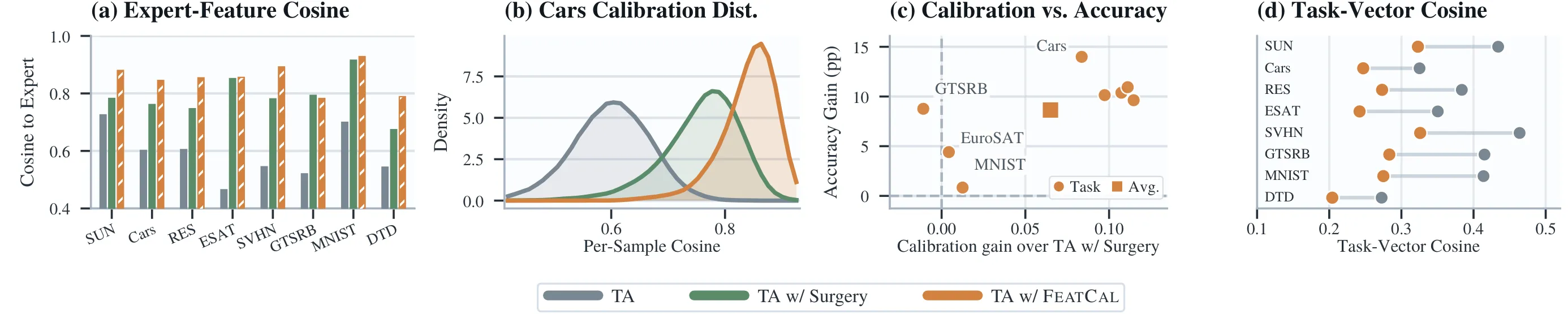
Figure 2. Feature-calibration diagnostics for TA on CLIP-ViT-B/32. (a) Task-wise final-feature cosine to experts; (b) per-sample cosine on Cars; (c) expert-cosine gain versus accuracy gain over TA w/ Surgery; (d) backbone task-vector cosine to same-task experts.
Feature-calibration diagnostics. Figure 2 tests whether TA w/ FeatCal gains coincide with final features closer to task experts. Panels (a) and (b) show larger expert cosine than Surgery in this setting: the macro average rises from 0.785 to 0.850 over TA w/ Surgery, and Stanford Cars has a mean per-sample gain of 0.084. This matches the intended mechanism because FeatCal calibrates the feature distribution reached by the deployed merged model. Panel (c) shows that expert-feature cosine is a diagnostic rather than a complete explanation: larger cosine gains often track accuracy gains, with an average -point gain over TA w/ Surgery, but EuroSAT and MNIST improve with small cosine changes, while GTSRB improves despite a slight decrease. Panel (d) highlights a feature-space and parameter-space mismatch: although FeatCal moves final features closer to experts, the calibrated backbone has lower same-task expert task-vector cosine than the TA baseline on every task. Thus, FeatCal calibrates the deployed feature distribution without bringing the backbone parameters into closer task-vector alignment, and the ProbSurgery comparison in Appendix J shows the same pattern with a stronger adapter baseline.
Table 5. Post-TA runtime at , excluding final evaluation. Speedup is relative to Surgery.
[2][4.35em][c]#1 #2
| CPU RSS | |||
|---|---|---|---|
| (Time) | (Wh) | (GiB) | |
| Surgery | 1.0x(217s) | 18.1 | 69.3 |
| ProbSurgery | 1.0x(224s) | 18.3 | 87.0 |
| FeatCal | 4.1x**(053s)** | 01.9 | 22.8 |
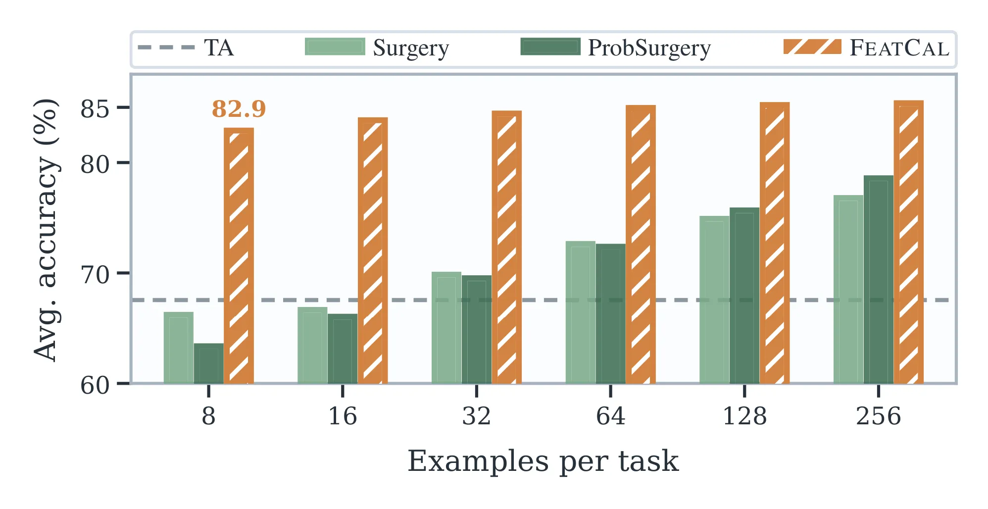
Figure 5. Sample Efficiency.
Sample efficiency and calibration cost. Figure 5 reports post-TA sample efficiency on CLIP-ViT-B/32 TA with matched per-task budgets . All methods start from the same Task Arithmetic model and differ only in the post-merging calibration stream. With examples per task, FeatCal already reaches average accuracy and then saturates near , while Surgery and ProbSurgery rise more slowly. Table 5 fixes : excluding final evaluation, the closed-form update takes 53s, faster than Surgery and faster than ProbSurgery, with lower GPU energy and much less peak CPU RSS. Together, FeatCal reaches most of its TA gain with few examples and keeps calibration cost low at . Full per-budget accuracy, resource averages, hardware, and logging details are in Appendix K.
Robustness to corrupted calibration data.
Table 6. 8-task TA accuracy under corrupted calibration. Avg. includes clean, Gaussian, blur, and fog.
| Method | Clean | Gauss. | Blur | Fog | Avg. |
|---|---|---|---|---|---|
| Task Arithmetic | 67.5 | -- | -- | -- | -- |
| w/ Surgery | 76.8 | 72.4 | 67.5 | 69.4 | 71.5 |
| w/ ProbSurgery | 79.1 | 73.2 | 65.8 | 68.2 | 71.6 |
| w/ FeatCal | 85.5 | 76.6 | 74.2 | 75.6 | 78.0 |
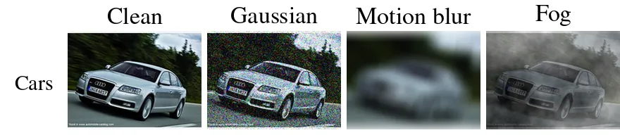
Figure 6. Calibration examples under corruptions.
We corrupt only the images used for post-merging calibration and evaluate on clean test sets from 8-task TA, isolating calibration data quality rather than test-time corruption robustness. Protocol details are in Appendix L.
FeatCal remains strongest in every reported setting, with a average over clean, Gaussian noise, motion blur, and fog, compared with for Surgery and for ProbSurgery. Corrupted runs remain below the clean reference, but the stable ordering in Figure 6 suggests that FeatCal extracts a reliable expert-feature calibration signal from imperfect data.
Ablation study.
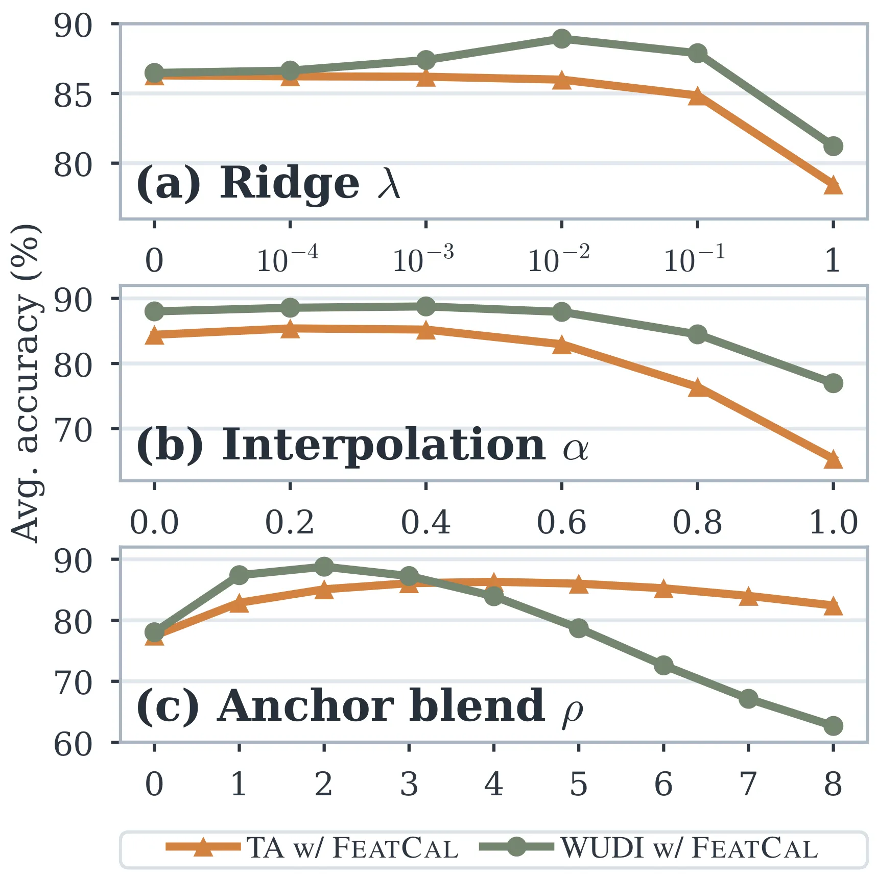
Figure 3. CLIP-ViT-B/32 TA coefficient sweeps.
Figure 3 reports single-factor sensitivity in the 8-task TA setting. FeatCal works best in a conservative calibration regime. Overly aggressive targets or regularization can degrade performance. The ridge sweep is flat over small positive values, so the closed-form solve is not tied to a narrow regularization choice, while very large ridge strength suppresses the update. The interpolation sweep has a sharper target-side tradeoff: small and medium values help, whereas the hard-expert endpoint can force local updates to absorb upstream drift that should be calibrated gradually across layers. The merged-base blend curve is most asymmetric: moderate extrapolation improves both upstream mergers, but large values push calibrated weights too far from the merged-base reference and especially hurt the WUDI variant. Overall, the ablation is a stability diagnostic with a broad conservative region rather than a single sharp optimum.
6. Conclusion
Feature drift frames post-merging calibration by showing how local mismatches can propagate through a merged model and affect outputs. FeatCal uses this signal by capturing features layer by layer and applying closed-form updates to linear modules, improving CLIP and FLAN-T5 mergers over Surgery and ProbSurgery in the main settings without adding modules at inference.
Acknowledgments
This work was supported by the Hong Kong RGC (TRS: T41-517/25-N; GRF: 15228325), ITC RAISe+ (RAI/24/1/086A), and the Research Institute for Generative Artificial Intelligence at PolyU.
_2026
BibTeX
@misc{gu-2026-featcal,
      title={FeatCal: Feature Calibration for Post-Merging Models},
      author={Yanggan Gu and Shuo Cai and Zihao Wang and Wenjun Wang and Yuanyi Wang and Pengkai Wang and Sirui Huang and Su Lu and Jianmin Wu and Hongxia Yang},
      year={2026},
      eprint={2605.13030},
      archivePrefix={arXiv},
      primaryClass={cs.LG},
      url={https://arxiv.org/abs/2605.13030},
}